Routing

Optimizing routing

As explained in architecture, Apache Pinot is a distributed system where different components have specific roles. Queries arrive at one of the brokers, that calculates which servers are going to participate in the query. In most clusters, a single server cannot hold all the segments, so each server has a partial view of the complete data. At the same time, segments are usually replicated on different servers in order to have high availability and better performance. In order to produce a complete result, the broker needs to calculate a subset of servers that contains all the segments that are required to resolve the query. Once this subset is calculated, the router uses a scatter and gather algorithm that sends the query to each server and then merges the partial results into the complete one.

There may be several subsets of servers that contain all the required segments. Any of them will return the correct result for the given query, but the subset used may affect the query performance. It is clear that the more servers participate in the query, the more CPUs, memory and IO can be used and therefore the better peak performance can be achieved. This is why, by default, brokers uniformly distribute the workload among as many servers as possible with balanced workload. Given that servers use segments as the minimum unit of work, the maximum parallelism is defined by the number of segments that are required to resolve the query.

What may be less clear is that the more servers participate in the query, the worse the tail latency (and even the resilience) will be. The reason is that the scatter and gather algorithm cannot produce a correct complete result until the partial results of all participating servers are collected. Therefore the latency of the query must be at least the higher latency of the servers participating and if any server crashes during the execution, the result merged in the broker may be incorrect. The more servers participate in a query, the higher the possibility to touch a server that requires some time to answer or to fail.

An easy-to-understand scenario is the impact of a full GC on a server. Let say a given query takes, on average, 30ms to execute. Depending on the JVM configuration that is used, a full GC may stop the process for a few hundreds of milliseconds, so if our query hits one server doing a full GC the latency will increase by at least one order or magnitude. Given that a correctly configured server shouldn't be stopped by full GCs very often, if to resolve this query a broker uses 3 servers, the possibility of hitting a server running a full GC is very small. Therefore, the tail latency of this query hitting 3 servers is expected to be close to 30ms. But if instead of 3 servers our query is spread on 30 servers, the possibility of hitting a server running a full GC increases significantly and therefore the tail latencies (p95, p99, etc) will increase.

To improve the tail latency, Apache Pinot provides two techniques at routing level:

• Reduce the query fanout by exploding data distribution.

• Reduce the query fanout by exploding data replication.

Reduce query fanout by exploding data distribution

As explained above, the broker must calculate the subset of servers that contains all the segments required to have a complete result. By default, the broker doesn't know anything about segments, so the subset of servers must contain all the segments in the table. This increases the number of servers that need to be asked. For example, in an extreme case where somehow the broker were able to know that only one segment was required, it could just ask one of the servers that contains that segment. By skipping servers that will not contain interesting data, the tail latency can be reduced without impacting the maximum peak performance.

Given that the number of segments may be large, the broker cannot store too much information per segment. One example of this is the bloom filters, which are used by servers to prune segments that will not contain relevant data to the given query. Given that the number of segments in a cluster can be quite large, brokers cannot afford to store them in memory and therefore bloom filters cannot be used to improve the rooting.

Instead, the user can inform Apache Pinot about specific patterns on which the data is actually distributed among segments. There are two patterns that can brokers can take advantage of and both can be used at the same time:

• Data ingested ordered by the optional time column.

• Data ingested partitioned by some column.

Data ingested ordered by the optional time column

When the schema defines a primary time column and data is ingested in approximate order by that column, brokers can optimize routing of queries that filter by that column. This is a common case for example when rows represent events (like logs, metrics, etc). As usual, Apache Pinot does not require events to be inserted in strict order. The closer the data distribution is to the strict order, the more selective this pruner will be but this technique can be used even when the data is not completely ordered.

To enable this optimization, segmentPartitionConfig must contain the time pruner type:

// Table config
{
  ...
  "routing": {
    "segmentPrunerTypes": ["time"]
  },
  ...
}

Data ingested partitioned by some column.

Apart from the ascending time, Apache Pinot can also take advantage of other distribution data patterns: Partition by segments. In order to use this feature, the table needs to be configured to use a partition function. Pinot will apply this function to each row in a segment and will store the set of partitions seen in the segment. Later, when a query is executed, Pinot will analyze the query in order to look for partition constraints. For example, when executing a query like select col1 from Table1 where col2 = 3, Pinot will calculate the partition associated with col2 = 3 and will prune segments that do not contain rows on that partition.

In order to make this pruning more efficient, segments should have the least number of partitions possible, which ideally is 1. More formally, given a function p, for all segments s, given any pair of rows r1 and r2, it should be true that p(r1) = p(r2). For example, in a table configured to have 3 partitions by memberId column, using modulo as the partition function, a segment that contains a row with memberId = 101 may also contain another row with memberId = 2 and another with memberId = 335, but it should not contain a row with memberId = 336 or memberId = 334.

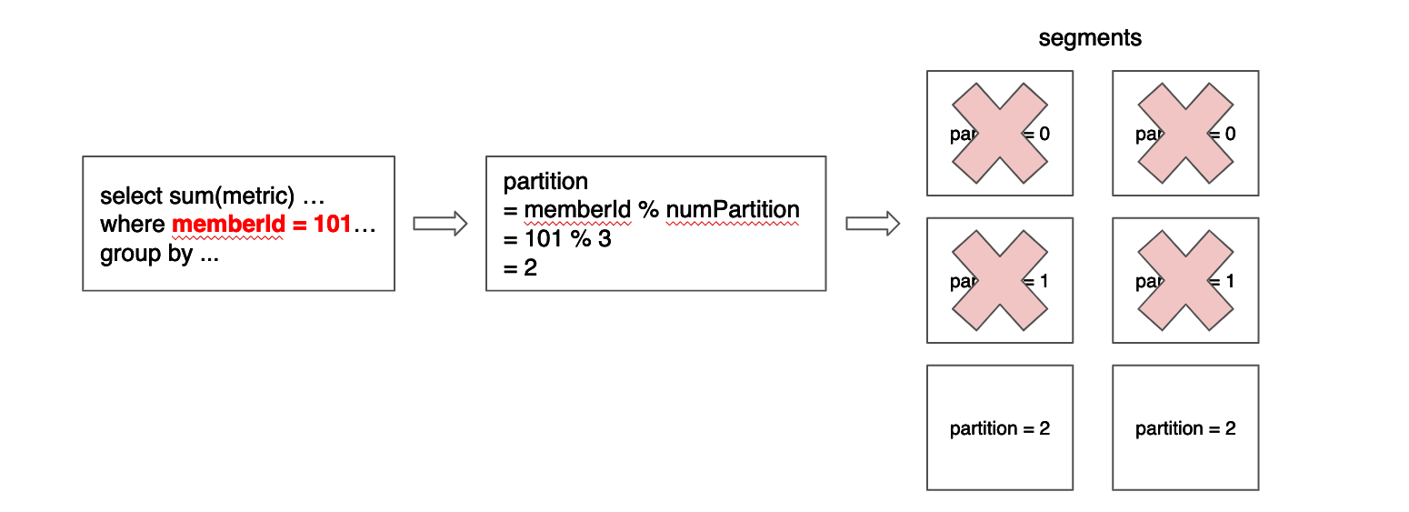
Data cannot always be partitioned by a dimension column or even when it is, not all queries can take advantage of the distribution. But when this optimization can be applied, a lot of segments can be pruned. The current implementation for partitioning only works for EQUALITY and IN filter (e.g. memberId = xx, memberId IN (x, y, z)). Below diagram gives the example of data partitioned on member id while the query includes an equality filter on member id.

Apache Pinot currently supports Modulo, Murmur, ByteArray and HashCode hash functions and partitioning can be enabled by setting the following configuration in the table config.

// Table config
{
  ...
  "tableIndexConfig": {
    ...
    "segmentPartitionConfig": {
      "columnPartitionMap": {
        "memberId": {
          "functionName": "Modulo",
          "numPartitions": 3
        }
      }
    },
    ...
  },
  ...
  "routing": {
    "segmentPrunerTypes": ["partition"]
  },
  ...
}

After setting the above config, data should be partitioned with the same partition function and number of partitions before running Pinot segment build and push job for offline push. Here's a scala UDF example of a partition function that Pinot understands, which is to be used for data partitioning.

private val NUM_PARTITIONS = 8
def getPartitionUdf: UserDefinedFunction = {
  udf((valueIn: Any) => {
    (murmur2(valueIn.toString.getBytes(UTF_8)) & Integer.MAX_VALUE) % NUM_PARTITIONS
  })
}

When applied correctly, partition information should be available in the segment metadata.

column.memberId.partitionFunction = Module
column.memberId.numPartitions = 3
column.memberId.partitionValues = 1

In order to maximize the partition pruning efficiency, it is important to reduce the number of partitions contained on each segment. Pinot will not move rows between segments to maximize partition efficiency, so when possible, rows should be correctly distribute before ingesting them into Pinot.

When using real-time tables, usually the input source can be used to do this partition. For example, one very usual input source in real-time tables is Kafka. In this case, in order to achieve maximum partition efficiency, Pinot and Kafka should use the same partition configuration.

When using offline tables, each input file should be crafted to contain rows on the same partition. Imagine we are creating a table from a list of CSV files. Ideally all rows in the csv should belong to the same partition. In the example above where we used modulo and 3 partitions, the value memberId = 101 will be associated with partition 2 (memberId % 3 = 2). Therefore to maximize the partition efficiency other rows in the same CSVv should have a memberId equal to 2, 5 or 104 but should not have values like 1, 3, 100 or 102.

Remember that Pinot does not impose a hard requirement here. It is fine if segments contain rows of more than one partition. What should be avoided is to have most segments associated with most partitions, given that in that case Pinot won't be actually able to prune most segments.

Reduce the query fanout by exploding data replication.

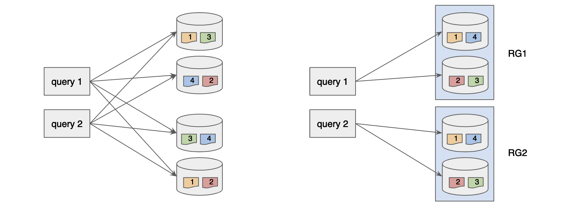
Although using partitions can drastically reduce the fanout, it only applies to specific queries and requires a specific data distribution between segments. The most consistent way to limit the fanout is to define replica group segment alignment. A Replica Group is a subset of servers that contains a ‘complete’ set of segments of a table. Once we assign the segment based on the replica group, each query can be answered by fanning out to a single replica group instead of all servers.

To use replica groups, the table configuration must be changed in the following ways:

• Replica groups must be declared in the InstanceAssignmentConfig section.

• RoutingConfig.instanceSelectorType must be changed to replicaGroup.

// Table config
{
  ...
  "instanceAssignmentConfigMap": {
    "OFFLINE": {
      ...
      "replicaGroupPartitionConfig": {
        "replicaGroupBased": true,
        "numReplicaGroups": 3,
        "numInstancesPerReplicaGroup": 4
      }
    }
  },
  ...
  "routing": {
    "instanceSelectorType": "replicaGroup"
  },
  ...
}

As seen above, you can use numReplicaGroups to control the number of replica groups (replications), and use numInstancesPerReplicaGroup to control the number of servers to span. For instance, let’s say that you have 12 servers in the cluster. Above configuration will generate 3 replica groups (numReplicaGroups=3), and each replica group will contain 4 servers (numInstancesPerPartition=4). In this example, each query will span to a single replica group (4 servers).

As seen above, replica groups give you the control on the number of servers to span for each query. When you try to decide the proper number of numReplicaGroups and numInstancesPerReplicaGroup, consider the trade-off between throughput and latency. Given a fixed number of servers, increasing numReplicaGroups factor while decreasing numInstancesPerReplicaGroup will make each query use less servers, which may reduce the possibility of one of them having a full GC. However, each server will need to process more number of segments per query, reducing the throughput, to the point that extreme values may even increase the average latency. Similarly, decreasing numReplicaGroups while increasing numInstancesPerReplicaGroup will make each query use more servers, increasing the possibility of one of them having a full GC but making each server process less number of segments per query. So, this number has to be decided based on the use case requirements.