Describes the literal relation operator in the multi-stage query engine.
The literal operator is used to define a constant value in the query. This operator may be generated by the multi-stage query engine when you use a constant value in a query.
Blocking nature
The literal operator is a blocking operator, but given its trivial nature it should not matter.
Implementation details
The literal operator is a simple operator that does not require any computation.
Hints
None
Stats
executionTimeMs
Type: Long
The summation of time spent by all threads executing the operator. This means that the wall time spent in the operation may be smaller that this value if the parallelism is larger than 1.
emittedRows
Type: Long
The number of groups emitted by the operator. It should always be one.
Explain attributes
None
Tips and tricks
Avoid very large literals
Take care when using very large literals (in the order hundreds of KBs), as they may need to be sent from brokers to servers and in general may introduce latencies in the parsing and query optimization.
Funnel Analysis
Apache Pinot supports a few funnel functions:
FunnelMaxStep
FunnelMaxStep evaluates user interactions within a specified time window to determine the furthest step reached in a predefined sequence of actions. By analyzing event timestamps and conditions set for each step, it identifies the maximum progression point for each user, ensuring that the sequence follows the configured order or other specific rules like strict timestamp increases or event uniqueness. This function is instrumental in funnel analysis, helping businesses and analysts understand user behavior, measure conversion rates, and identify potential drop-offs in critical user journeys.
Similar to FunnelMaxStep , this function returns an array which reflects the matching status for the steps.
FunnelCompleteCount
This function evaluates all funnel events and returns how many times the user has completed the full steps.
Window
Describes the window relational operator in the multi-stage query engine.
The window operator is used to define a window over which to perform calculations.
This page describes the window operator defined in the relational algebra used by multi-stage queries. This operator is generated by the multi-stage query engine when you window functions in a query. You can read more about window functions in the reference documentation.
Unlike the , which will output one row per group, the window operator will output as many rows as input rows.
Implementation details
Transform
Describes the transform relation operator in the multi-stage query engine.
The transform operator is used to apply a transformation to the input data. They may filter out columns or add new ones by applying functions to the existing columns. This operator is generated by the multi-stage query engine when you use a SELECT clause in a query, but can also be used to implement other transformations.
Implementation details
Transform operators apply some transformation functions to the input data received from upstream. The cost of the transformation usually depends on the complexity of the functions applied, but comparing to other operators, it is usually not very high.
Mailbox receive
Describes the mailbox receive operator in the multi-stage query engine.
The mailbox receive operator is the operator that receives the data from the mailbox send operator. This is not an actual relational operator but a Pinot extension used to receive data from other stages.
Implementation details
Stages in the multi-stage query engine are executed in parallel by different workers. Workers send data to each other using mailboxes. The number of mailboxes depends on the send operator parallelism, the receive operator parallelism and the distribution being used. At worse, there is one mailbox per worker pair, so if the upstream send operator has a parallelism of S and the receive operator has a parallelism of R, there will be S * R mailboxes.
Multi stage query
Learn more about multi-stage query engine and how to troubleshoot issues.
The general explanation of the multi-stage query engine is provided in the reference documentation. This section provides a deep dive into the multi-stage query engine. Most of the concepts explained here are related to the internals of the multi-stage query engine and users don't need to know about them in order to write queries. However, understanding these concepts can help you to take advantage of the engine's capabilities and to troubleshoot issues.
By default, these mailboxes are GRPC channels, but when both workers are in the same server, they can use shared memory and therefore a more efficient on heap mailbox is used.
The mailbox receive operator pulls data from these mailboxes and sends it to the downstream operator.
Blocking nature
The mailbox receive operator is a streaming operator. It emits the blocks of rows as soon as they are received from the upstream operator.
It is important to notice that the mailbox receive operator tries to be fair when reading from multiple workers.
Hints
None
Stats
executionTimeMs
Type: Long
The summation of time spent by all threads executing the operator. This means that the wall time spent in the operation may be smaller that this value if the parallelism is larger than 1.
emittedRows
Type: Long
The number of groups emitted by the operator. This operator should always emit as many rows as its upstream operator.
fanIn
Type: Long
How many workers are sending data to this operator.
inMemoryMessages
Type: Long
How many messages have been received in heap format by this mailbox. Receiving in heap messages is more efficient than receiving them in raw format, as the messages do not need to be serialized and deserialized and no network transfer is needed.
rawMessages
Type: Long
How many messages have been received in raw format and therefore serialized by this mailbox. Receiving in heap messages is more efficient than receiving them in raw format, as the messages do not need to be serialized and deserialized and no network transfer is needed.
deserializedBytes
Type: Long
How many bytes have been deserialized by this mailbox. A high number here indicates that the mailbox is receiving a lot of data from other servers, which is expensive in terms of CPU, memory and network.
deserializeTimeMs
Type: Long
How long it took to deserialize the raw messages sent to this mailbox. This time is not wall time, but the sum of the time spent by all threads deserializing messages.
Take into account that this time does not include the impact on the network or the GC.
downstreamWaitMs
Type: Long
How much time this operator has been blocked waiting while offering data to be consumed by the downstream operator. A high number here indicates that the downstream operator is slow and may be a bottleneck. For example, usually the receive operator that is the left input of a join operator has a high value here, as the join needs to consume all the messages from the right input before it can start consuming the left input.
upstreamWaitMs
Type: Long
How much time this operator has been blocked waiting for more data to be sent by the upstream (send) operator. A high number here indicates that the upstream operator is slow and may be a bottleneck. For example, blocking operators like aggregations, sorts, joins or window functions require all the data to be received before they can start emitting a result, so having them as upstream operators of a mailbox receive operator can lead to high values here.
Explain attributes
Given that the mailbox receive operator is a meta-operator, it is not actually shown in the explain plan. Instead, a single PinotLogicalExchange or PinotLogicalSortExchange is shown in the explain plan. This exchange explain node is the logical representation of a pair of send and receive operators.
See the mailbox send operator to understand the attributes of the exchange explain node.
Window operators take a single input relation and apply window functions to it. For each input row, a window of rows is calculated and one or many aggregations are applied to it.
In general window operator are expensive in terms of CPU and memory usage, but they open the door to a wide range of analytical queries.
Blocking nature
The window operator is a blocking operator. It needs to consume all the input data before emitting the result.
Hints
Window hints are configured with the windowOptions hint, which accepts as argument a map of options and values.
For example:
max_rows_in_window
Type: Integer
Default: 1048576
Max rows allowed to cache the rows in window for further processing.
window_overflow_mode
Type: THROW or BREAK
Default: 'THROW'
Mode when window overflow happens, supported values:
THROW: Break window cache build process, and throw exception, no further WINDOW operation performed.
BREAK: Break window cache build process, continue to perform WINDOW operation, results might be partial.
Stats
executionTimeMs
Type: Long
The summation of time spent by all threads executing the operator. This means that the wall time spent in the operation may be smaller that this value if the parallelism is larger than 1. This number is affected by the number of received rows and the complexity of the window function.
emittedRows
Type: Long
The number of groups emitted by the operator. A large number of emitted rows can indicate that the query is not well optimized.
Unlike the aggregate operator, which will output one row per group, the window operator will output as many rows as input rows.
maxRowsInWindowReached
Type: Boolean
This attribute is set to true if the maximum number of rows in the window has been reached.
Explain attributes
The window operator is represented in the explain plan as a LogicalWindow explain node.
window#
Type: Expression
The window expressions used by the operator. There may be more than one of these attributes depending on the number of window functions used in the query, although sometimes multiple window function clauses in SQL can be combined into a single window operator.
The expression may use indexed columns ($0, $1, etc) that represent the columns of the virtual row generated by the upstream.
The transform operator is a streaming operator. It emits the blocks of rows as soon as they are received from the upstream operator.
Hints
None
Stats
executionTimeMs
Type: Long
The summation of time spent by all threads executing the operator. This means that the wall time spent in the operation may be smaller that this value if the parallelism is larger than 1.
emittedRows
Type: Long
The number of groups emitted by the operator.
Explain attributes
The transform operator is represented in the explain plan as a LogicalProject explain node.
This explain node has a list of attributes that represent the transformations applied to the input data. Each attribute has a name and a value, which is the expression used to generate the column.
For example:
Is saying that the output of the operator has three columns:
userUUID is the 7th column in the virtual row projected by LogicalTableScan, which corresponds to the userUUID column in the table.
deviceOS is the 5th column in the virtual row projected by LogicalTableScan, which corresponds to the deviceOS column in the table.
EXPR$2 is the result of the SUBSTRING($4, 0, 2) expression applied to the 5th column in the virtual row projected by LogicalTableScan. Given we know that the 5th column is deviceOS, we can infer that EXPR$2 is the first two characters of the deviceOS column.
Tips and tricks
None
SELECT
/*+ windowOptions(option1='value1', option2='value2') */
col1, SUM(intCol) OVER() as sum FROM table
The multi-stage query engine uses a set of operators to process the query. These operators are based on relational algebra, with some modifications to better fit the distributed nature of the engine.
These operators are the execution units that Pinot uses to execute a query. The operators are executed in a pipeline with tree structure, where each operator consumes the output of the previous operators (also known as upstreams).
Users do not directly specify these operators. Instead they write SQL queries that are translated into a logical plan, which is then transformed into different operators. The logical plan can be obtained using explaining a query, while there is no way to get the operators directly. The closest thing to the operators that users can get is the multi-stage stats output.
Operators vs SQL clauses
These operators are generated from the SQL query that you write, but even they are similar, there is not a one-to-one mapping between the SQL clauses and the operators. Some SQL clauses generate multiple operators, while some operators are generated by multiple SQL clauses.
Operators vs explain plan nodes
Operators and explain plan nodes are closer than SQL clauses and operators. Although most explain plan nodes can be directly mapped to an operator, there are some exceptions:
Each PinotLogicalExchange and each PinotLogicalSortExchange explain node is materialized into a pair of and operators.
All plan nodes that belong to the same leaf stage are executed in the operator.
In general terms, the operators are the execution units that Pinot uses to execute a query and are also known as the multi-stage physical plan, while the explain plan nodes are logical plans. The difference between the two is that the operators can be actually executed, while the explain plan nodes are the logical representation of the query plan.
List of operators
The following is a list of operators that are used by the multi-stage query engine:
Filter
Describes the filter relation operator in the multi-stage query engine.
The filter operator is used to filter rows based on a condition.
This page describes the filter operator defined in the relational algebra used by multi-stage queries. This operator is generated by the multi-stage query engine when you use the where, having or sometimes on clauses.
Implementation details
Filter operations apply a predicate to each row and only keep the rows that satisfy the predicate.
It is important to notice that filter operators can only be optimized using indexes when they are executed in the leaf stage. The reason for that is that the intermediate stages don't have access to the actual segments. This is why the engine will try to push down the filter operation to the leaf stage whenever possible.
As explained in , the explain plan in the multi-stage query engine does not indicate whether indexes are used or not.
Blocking nature
The filter operator is a streaming operator. It emits the blocks of rows as soon as they are received from the upstream operator.
Hints
None
Stats
executionTimeMs
Type: Long
The summation of time spent by all threads executing the operator. This means that the wall time spent in the operation may be smaller that this value if the parallelism is larger than 1. This number is affected by the number of received rows and the complexity of the predicate.
emittedRows
Type: Long
The number of groups emitted by the operator. A large number of emitted rows may not be problematic, but indicates that the predicate is not very selective.
Explain attributes
The filter operator is represented in the explain plan as a LogicalFilter explain node.
condition
Type: Expression
The condition that is being applied to the rows. The expression may use indexed columns ($0, $1, etc), functions and literals. The indexed columns are always 0-based.
For example, the following explain plan:
Is saying that the filter is applying the condition $5 > 2 which means that only the rows where the 6th column is greater than 2 will be emitted. In order to know which column is the 6th, you need to look at the schema of the table scanned.
Tips and tricks
How to know if indexes are used
As explained in , the explain plan in the multi-stage query engine does not directly indicate whether indexes are used or not.
Apache Pinot contributors are working on improving this, but it is not yet available. Meanwhile, we need an indirect approach to get that information.
First, we need to know on which stage the filter is being used. If the filter is being used in an intermediate stage, then the filter is not using indexes. In order to know the stage, you can extract stages as explained in .
But what about the leaf filters executed in the stage? Not all filters in the leaf stage can use indexes. The only way to know if the filter is using indexes is to use single-stage explain plan. In order to do so you need to transform the leaf stage into a single-stage query. This is a manual process that can be tedious but ends up not being so difficult once you get used to it.
See for more information.
Explain
Learn more about multi-stage explain plans and how to interpret them.
Multi-stage plans are a bit more complex than single-stage plans. This page explains how to interpret multi-stage explain plans.
As explained in Explaining multi-stage queries, you can use the EXPLAIN PLAN syntax to obtain the logical plan of a query. There are different formats for the output of the EXPLAIN PLAN command, but all of them represent the logical plan of the query.
The query
Can produce the following output:
We can see that each node in the tree represents an operation that is executed in the query and each operator has some attributes. For example the LogicalJoin operator has a condition attribute that specifies the join condition and a joinType. Although some of the attributes shown are easy to understand, some of them may require a bit more explanation.
In our example we can see that the LogicalTableScan operator has a table attribute that indicates the table being scanned. The table is represented as a list with two elements: the first one is the schema name (default by default) and the second one is the table name. Attributes like offset and fetch in the LogicalSort operator are also easy to understand. But once we start to see expressions and references like $2 things start to be more complex.
These indexed references are used to reference the positions into the input row for each operator. In order to understand these references we need to look at the operator's children and see which attributes are being referenced. That usually requires going to the leaf operators and seeing which attributes are being generated.
For example, the LogicalTableScan always returns the whole row of the table, so the attributes are the columns of the table. In our example:
We can see that the result of the LogicalTableScan operator is processed by a LogicalProject operator that is selecting the columns o_custkey and o_shippriority. This LogicalProject operator is generating a row with two columns. $5 and $10 are the indexes of the column o_custkey and o_shippriority in the row generated by the LogicalTableScan. Then we can see a PinotLogicalExchange operator that is sending the result to the LogicalJoin
The LogicalJoin operator is receiving the rows from the two stages upstream. It is not clearly said anywhere, but the virtual row seen by the join operator is the concatenation of the rows sent by the first stage (aka left hand size) plus the rows sent by the second stage (aka right hand side).
The first stage is sending the c_address and c_custkey columns and the second stage is sending the o_custkey and o_shippriority columns. Therefore the join operator is consuming a row with the columns [c_address, c_custkey, o_custkey, o_shippriority]. The LogicalJoin operator is joining the rows using the condition =($1, $2), which means that it is joining the rows using the c_custkey and o_custkey columns and comparing them by equality. LogicalJoin can generate new rows, but does not modify the virtual columns. Therefore this join is sending rows with the columns [c_address, c_custkey, o_custkey, o_shippriority] to its downstream.
This downstream is the LogicalProject operator that is selecting the columns $0 and $3 from the rows sent by the join operator. Therefore the resulting row contains the columns c_address and o_shippriority.
The rest of the operators are easier to read. Something that can be surprising is the LogicalSort operator. In the SQL query used as example there was no order by, but the LogicalSort operator is present in the plan. This is because in relational algebra a sort is always needed to limit the rows. In this case the LogicalSort operator is limiting the rows to 10 without specifying a sort condition, so it is not really sorting the rows (which may be expensive). The corollary is that a LogicalSort operator does not imply that an actual sort is being executed.
Understanding Stages
Learn more about multi-stage stages and how to extract stages from query plans.
Deep dive into stages
As explained in the Multi-stage query engine reference documentation, the multi-stage query engine breaks down a query into multiple stages. Each stage corresponds to a subset of the query plan and is executed independently. Stages are connected in a tree-like structure where the output of one stage is the input to another stage. The stage that is at the root of the tree sends the final results to the client. The stages that are at the leaves of the tree read from the tables. The intermediate stages process the data and send it to the next stage.
When the broker receives a query, it generates a query plan. This is a tree-like structure where each node is an operator. The plan is then optimized, moving and changing nodes to generate a plan that is semantically equivalent (it returns the same rows) but more efficient. During this phase the broker colors the nodes of the plan, assigning them to a stage. The broker also assigns a parallelism to each stage and defines which servers are going to execute each stage. For example, if a stage has a parallelism of 10, then at most 10 servers will execute that stage in parallel. One single server can execute multiple stages in parallel and it can even execute multiple instances of the same stage in parallel.
Stages are identified by their stage ID, which is a unique identifier for each stage. In the current implementation the stage ID is a number and the root stage has a stage ID of 0, although this may change in the future.
The current implementation has some properties that are worth mentioning:
The leaf stages execute a slightly modified version of the single-stage query engine. Therefore these stages cannot execute joins or aggregations, which are always executed in the intermediate stages.
Intermediate stages execute operations using a new query execution engine that has been created for the multi-stage query engine. This is why some of the functions that are supported in the single-stage query engine are not supported in the multi-stage query engine and vice versa.
An intermediate stage can only have one join, one window function or one set operation. If a query has more than one of these operations, the broker will create multiple stages, each with one of these operations.
Extracting Stages from Query Plans
As explained in , you can use the EXPLAIN PLAN syntax to obtain the logical plan of a query. This logical plan can be used to extract the stages of the query.
For example, if the query is:
A possible output of the EXPLAIN PLAN command is:
As it happens with all queries, the logical plan forms a tree-like structure. In this default explain format, the tree-like structure is represented with indentation. The root of the tree is the first line, which is the last operator to be executed and marks the root stage. The boundary between stages are the PinotLogicalExchange operators. In the example above, there are four stages:
The root stage starts with the LogicalSort operator in the root of operators and ends with the PinotLogicalSortExchange operator. This is the last stage to be executed and the only one that is executed in the broker, which will directly send the result to the client once it is computed.
The next stage starts with this PinotLogicalSortExchange operator and includes the LogicalSort operator, the LogicalProject operator, the LogicalJoin
Now that we have identified the stages, we can understand what each stage is doing by .
Aggregate
Describes the aggregate relation operator in the multi-stage query engine.
The aggregate operator is used to perform calculations on a set of rows and return a single row of results.
This page describes the aggregate operator defined in the relational algebra used by multi-stage queries. This operator is generated by the multi-stage query engine when you use aggregate functions in a query either with or without a group by clause.
Implementation details
Querying Pinot
Learn how to query Pinot using SQL
SQL Interface
Pinot provides a SQL interface for querying, which uses the Calcite SQL parser to parse queries and the MYSQL_ANSI dialect. For details on the syntax, see the the . To find supported SQL operators, see .
Intersect
Describes the intersect relation operator in the multi-stage query engine.
The intersect operator is a relational operator that combines two relations and returns the common rows between them. The operator is used to find the intersection of two or more relations, usually by using the SQL INTERSECT operator.
Although it is accepted by the parser, the ALL modifier is currently ignored. Therefore INTERSECT and INTERSECT ALL are equivalent. This issue has been reported in
Minus
Describes the minus relation operator in the multi-stage query engine.
The minus operator is used to subtract the result of one query from another query. This operator is used to find the difference between two sets of rows, usually by using the SQL EXCEPT operator.
Although it is accepted by the parser, the ALL modifier is currently ignored. Therefore EXCEPT and EXCEPT ALL are equivalent. This issue has been reported in
explain plan for
select customer.c_address, orders.o_shippriority
from customer
join orders
on customer.c_custkey = orders.o_custkey
limit 10
, which means to use the hash of the first column returned by
LogicalProject
. As we saw before, that first column is the
o_custkey
column, so the rows are distributed by the
o_custkey
column.
operator and the two
PinotLogicalExchange
operators. This stage clearly is not a root stage and it is not reading data from the segments, so it is not a leaf stage. Therefore it has to be an intermediate stage.
The join has two children, which are the PinotLogicalExchange operators. In this specific case, both sides are very similar. They start with a PinotLogicalExchange operator and end with a LogicalTableScan operator. All stages that end with a LogicalTableScan operator are leaf stages.
Aggregate operations may be expensive in terms of memory, CPU and network usage. As explained in understanding stages, the multi-stage query engine breaks down the query into multiple stages and each stage is then executed in parallel on different workers. Each worker processes a subset of the data and sends the results to the coordinator which then aggregates the results. When possible, the multi-stage query engine will try to apply a divide-and-conquer strategy to reduce the amount of data that needs to be processed in the coordinator stage.
For example if the aggregation function is a sum, the engine will try to sum the results of each worker before sending the partial result to the coordinator, which would then sum the partial results in order to get the final result. But some aggregation functions, like count(distinct), cannot be computed in this way and require all the data to be processed in the coordinator stage.
In Apache Pinot 1.1.0, the multi-stage query engine always keeps the data in memory. This means that the amount of memory used by the engine is proportional to the number of groups generated by the group by clause and the amount of data that needs to be kept for each group (which depends on the aggregation function).
Even when the aggregation function is a simple count, which only requires to keep a long for each group in memory, the amount of memory used can be high if the number of groups is high. This is why the engine limits the number of groups. By default, this limit is 100.000, but this can be changed by providing hints.
Blocking nature
The aggregate operator is a blocking operator. It needs to consume all the input data before emitting the result.
Hints
num_groups_limit
Type: Integer
Default: 100.000
Defines the max number of groups that can be created by the group by clause. If the number of groups exceeds this limit, the query will not fail but will stop the execution.
Example:
is_partitioned_by_group_by_keys
Type: Boolean
Default: false
If set to true, the engine will consider that the data is already partitioned by the group by keys. This means that the engine will not need to shuffle the data to group them by the group by keys and the coordinator stage will be able to compute the final result without needing to merge the partial results.
Caution: This hint should only be used if the data is already partitioned by the group by keys. There is no check to verify that the data is indeed partitioned by the group by keys and using this hint when the data is not partitioned by the group by keys will lead to incorrect results.
Example:
is_skip_leaf_stage_group_by
Type: Boolean
Default: false
If set to true, the engine will not push down the aggregate into the leaf stage. In some situations, it could be wasted effort to do group-by on leaf, eg: when cardinality of group by column is very high.
Example:
max_initial_result_holder_capacity
Type: Integer
Default: 10.000
Defines the initial capacity of the result holder that stores the intermediate results of the aggregation. This hint can be used to reduce the memory usage of the engine by setting a value close to the expected number of groups. It is usually recommended to not change this hint unless you know that the expected number of groups is much lower than the default value.
Example:
Stats
executionTimeMs
Type: Long
The summation of time spent by all threads executing the operator. This means that the wall time spent in the operation may be smaller that this value if the parallelism is larger than 1. Remember that this value is affected by the number of received rows and the complexity of the aggregation function.
emittedRows
Type: Long
The number of groups emitted by the operator. A large number of emitted rows can indicate that the query is not well optimized.
Remember that the number of groups is limited by the num_groups_limit hint and a large number of groups can lead to high memory usage and slow queries.
numGroupsLimitReached
Type: Boolean
This stat is set to true when the number of groups exceeds the limit defined by the num_groups_limit hint. In that case, the query will not fail but will return partial results, which will be indicated by the global partialResponse stat.
Explain attributes
The aggregate operator is represented in the explain plan as a LogicalAggregate explain node.
Remember that these nodes appear in pairs: First in one stage where the aggregation is done in parallel and then in the upstream stage where the partial results are merged.
group
Type: List of Integer
The list of columns used in the group by clause. These numbers are 0-based column indexes on the virtual row projected by the upstream.
For example the explain plan:
Is saying that the group by clause is using the column with index 6 in the virtual row projected by the upstream. Given in this case that row is generated by a table scan, the column with index 6 is the 7th column in the table as defined in its schema.
agg#N
Type: Expression
The aggregation functions applied to the columns. There may be multiple agg#N attributes, each one representing a different aggregation function.
For example the explain plan:
Has two aggregation functions: COUNT() and MAX(). The second is applied to the column with index 5 in the virtual row projected by the upstream. Given in this case that row is generated by a table scan, the column with index 5 is the 6th column in the table as defined in its schema.
Tips and tricks
Try to not use aggregation functions that cannot be parallelized
For example, it is recommended to use one of the different hyperloglog flavor instead of count(distinct) when the cardinality of the data or their size.
For example, it is cheaper to execute count(distinct) on an int column with 1000 distinct values than on a column that stores very long strings, even if the number of distinct values is the same.
Pinot 1.0
In Pinot 1.0, the multi-stage query engine supports inner join, left-outer, semi-join, and nested queries out of the box. It's optimized for in-memory process and latency. For more information, see how to enable and use the multi-stage query engine.
Pinot also supports using simple Data Definition Language (DDL) to insert data into a table from file directly. For details, see programmatically access the multi-stage query engine. More DDL supports will be added in the future. But for now, the most common way for data definition is using the Controller Admin API.
Note: For queries that require a large amount of data shuffling, require spill-to-disk, or are hitting any other limitations of the multi-stage query engine (v2), we still recommend using Presto.
Identifier vs Literal
In Pinot SQL:
Double quotes(") are used to force string identifiers, e.g. column names
Single quotes(') are used to enclose string literals. If the string literal also contains a single quote, escape this with a single quote e.g '''Pinot''' to match the string literal 'Pinot'
Misusing those might cause unexpected query results, like the following examples:
WHERE a='b' means the predicate on the column a equals to a string literal value 'b'
WHERE a="b" means the predicate on the column a equals to the value of the column b
If your column names use reserved keywords (e.g. timestamp or date) or special characters, you will need to use double quotes when referring to them in queries.
Note: Define decimal literals within quotes to preserve precision.
The current implementation consumes the whole right input relation first and stores the rows in a set. Then it consumes the left input relation one block at a time. Each time a block of rows is read from the left input relation, the operator checks if the rows are in the set of rows from the right input relation. All unique rows that are in the set are added to a new partial result block. Once the whole left input block is analyzed, the operator emits the partial result block.
This process is repeated until all rows from the left input relation are processed.
In pseudo-code, the algorithm looks like this:
Blocking nature
The intersect operator is a semi-blocking operator that first consumes the right input relation in a blocking fashion and then consumes the left input relation in a streaming fashion.
Hints
None
Stats
executionTimeMs
Type: Long
The summation of time spent by all threads executing the operator. This means that the wall time spent in the operation may be smaller that this value if the parallelism is larger than 1.
emittedRows
Type: Long
The number of groups emitted by the operator.
Explain attributes
The intersect operator is represented in the explain plan as a LogicalIntersect explain node.
all
Type: Boolean
This attribute is used to indicate if the operator should return all the rows or only the distinct rows.
Although it is accepted in SQL, the all attribute is not currently used in the intersect operator. The returned rows are always distinct. This issue has been reported in #13126
Tips and tricks
The order of input relations matter
The intersect operator has a memory footprint that is proportional to the number of unique rows in the right input relation. It also consumes the right input relation in a blocking fashion while the left input relation is consumed in a streaming fashion.
This means that:
In case any of the input relations is significantly larger than the other, it is recommended to use the smaller relation as the right input relation.
In case one of the input is blocking and the other is not, it is recommended to use the blocking relation as the right input relation.
These two hints can be contradictory, so it is up to the user to decide which one to follow based on the specific query pattern. Remember that you can use the stage stats to check the number of rows emitted by each of the inputs and adjust the order of the inputs accordingly.
The minus operator is a semi-blocking operator that first consumes the right input relation in a blocking fashion and then consumes the left input relation in a streaming fashion.
The current implementation consumes the whole right input relation first and stores the rows in a set. Then it consumes the left input relation one block at a time. Each time a block of rows is read from the left input relation, the operator checks if the rows are in the set of rows from the right input relation. All unique rows that are not in the set are added to a new partial result block. Once the whole left input block is analyzed, the operator emits the partial result block.
This process is repeated until all rows from the left input relation are processed.
Blocking nature
The minus operator is a semi-blocking operator that first consumes the right input relation in a blocking fashion and then consumes the left input relation in a streaming fashion.
In pseudo-code, the algorithm looks like this:
Hints
None
Stats
executionTimeMs
Type: Long
The summation of time spent by all threads executing the operator. This means that the wall time spent in the operation may be smaller that this value if the parallelism is larger than 1.
emittedRows
Type: Long
The number of groups emitted by the operator.
Explain attributes
The minus operator is represented in the explain plan as a LogicalMinus explain node.
all
Type: Boolean
This attribute is used to indicate if the operator should return all the rows or only the distinct rows.
Although it is accepted in SQL, the all attribute is not currently used in the minus operator. The returned rows are always distinct. This issue has been reported in #13127
Tips and tricks
Memory pressure
The minus operator ends up having to store all unique rows from both input relations in memory. This can lead to memory pressure if the input relations are large and have a high number of unique rows.
The order of input relations matter
Although the minus operator ends up adding all unique rows from both input relations to a set, the order of input relations matters. While the right input relation is consumed in a blocking fashion, the left input relation is consumed in a streaming fashion. Therefore the latency of the whole query could be improved if the left input relation is producing values in streaming fashion.
In case one of the inputs is blocking and the other is not, it is recommended to use the blocking relation as the right input relation.
//default to limit 10
SELECT *
FROM myTable
SELECT *
FROM myTable
LIMIT 100
SELECT "date", "timestamp"
FROM myTable
SELECT COUNT(*), MAX(foo), SUM(bar)
FROM myTable
SELECT MIN(foo), MAX(foo), SUM(foo), AVG(foo), bar, baz
FROM myTable
GROUP BY bar, baz
LIMIT 50
SELECT MIN(foo), MAX(foo), SUM(foo), AVG(foo), bar, baz
FROM myTable
GROUP BY bar, baz
ORDER BY bar, MAX(foo) DESC
LIMIT 50
SELECT COUNT(*)
FROM myTable
WHERE foo = 'foo'
AND bar BETWEEN 1 AND 20
OR (baz < 42 AND quux IN ('hello', 'goodbye') AND quuux NOT IN (42, 69))
SELECT COUNT(*)
FROM myTable
WHERE foo IS NOT NULL
AND foo = 'foo'
AND bar BETWEEN 1 AND 20
OR (baz < 42 AND quux IN ('hello', 'goodbye') AND quuux NOT IN (42, 69))
SELECT *
FROM myTable
WHERE quux < 5
LIMIT 50
SELECT foo, bar
FROM myTable
WHERE baz > 20
ORDER BY bar DESC
LIMIT 100
SELECT foo, bar
FROM myTable
WHERE baz > 20
ORDER BY bar DESC
LIMIT 50, 100
SELECT COUNT(*)
FROM myTable
WHERE REGEXP_LIKE(airlineName, '^U.*')
GROUP BY airlineName LIMIT 10
SELECT
CASE
WHEN price > 30 THEN 3
WHEN price > 20 THEN 2
WHEN price > 10 THEN 1
ELSE 0
END AS price_category
FROM myTable
SELECT
SUM(
CASE
WHEN price > 30 THEN 30
WHEN price > 20 THEN 20
WHEN price > 10 THEN 10
ELSE 0
END) AS total_cost
FROM myTable
SELECT COUNT(*)
FROM myTable
GROUP BY DATETIMECONVERT(timeColumnName, '1:MILLISECONDS:EPOCH', '1:HOURS:EPOCH', '1:HOURS')
SELECT *
FROM myTable
WHERE UID = 'c8b3bce0b378fc5ce8067fc271a34892'
HashSet<Row> rightRows = new HashSet<>();
Block rightBlock = rightInput.nextBlock();
while (rightBlock is not EOS) {
rightRows.addAll(rightBlock.getRows());
rightBlock = rightInput.nextBlock();
}
Block leftBlock = leftInput.nextBlock();
while (leftBlock is not EOS) {
Block partialResultBlock = new Block();
for (Row row : leftBlock.getRows()) {
if (rightRows.remove(row)) {
partialResultBlock.add(row);
}
}
emit partialResultBlock;
leftBlock = leftInput.nextBlock();
}
emit EOS
HashSet<Row> rightRows = new HashSet<>();
Block rightBlock = rightInput.nextBlock();
while (rightBlock is not EOS) {
rightRows.addAll(rightBlock.getRows());
rightBlock = rightInput.nextBlock();
}
Block leftBlock = leftInput.nextBlock();
while (leftBlock is not EOS) {
Block partialResultBlock = new Block();
for (Row row : leftBlock.getRows()) {
if (rightRows.add(row)) {
partialResultBlock.add(row);
}
}
emit partialResultBlock;
leftBlock = leftInput.nextBlock();
}
emit EOS
Sort or limit
Describes the sort or limit relation operator in the multi-stage query engine.
The sort or limit operator is used to sort the input data, limit the number of rows emitted by the operator or both. This operator is generated by the multi-stage query engine when you use an order by, limit or offset operation in a query.
Implementation details
Blocking nature
Hints
None
Stats
executionTimeMs
Type: Long
The summation of time spent by all threads executing the operator. This means that the wall time spent in the operation may be smaller that this value if the parallelism is larger than 1.
emittedRows
Type: Long
The number of groups emitted by the operator.
Explain attributes
The sort or limit operator is represented in the explain plan as a LogicalSort explain node.
sort#
Type: Expression
The sort expressions used by the operator. There is one of these attributes per sort expression. The first one is sort0, the second one is sort1, and so on.
The value of this attribute is the expression used to sort the data and may contain indexed columns ($0, $1, etc) that represent the columns of the virtual row generated by the upstream.
For example, the following plan:
Is saying that the rows are sorted first by the column with index 0 and then by the column with index 2 in the virtual row generated by the upstream. That column is generated by a projection whose first column (index 0) is userUUID, the second (index 1) is deviceOS and third (index 2) is the result of the SUBSTRING($4, 0, 2) expression. As we know $4 in this project is deviceOS, we can infer that the third column is the first two characters of the deviceOS column.
dir#
Type: ASC or DESC
The direction of the sort. There is one of these attributes per sort expression.
fetch
Type: Long
The number of rows to emit. This is the equivalent to LIMIT in SQL. Remember that the limit can be applied without sorting, in which case the order on which the rows are emitted is undefined.
offset
Type: Long
The number of rows to skip before emitting the rows. This is the equivalent to OFFSET in SQL.
Tips and tricks
Limit and offset can prevent filter pushdown
In SQL, usually limit and offset are used in the last stage of the query. But when being used in the middle of the query (like in a subquery or a CTE), it can prevent filter pushdown optimization.
For example, imagine the following query:
This query may generate the plan:
We can see that the filter deviceOS = 'windows' is pushed down to the leaf stage. This reduce the amount of data that needs to be scanned and can improve the query performance, specially if there is an inverted index in the deviceOS column.
But if we modify the query to add a limit to the userAttributes table scan:
The generated plan will be:
Here we can see that the filter deviceOS = 'windows' is not pushed down leaf stage, which means that the engine will need to scan all the data in the userAttributes table and then apply the filter.
The reason why the filter is not pushed down is that the limit operation must be applied before the filter in order to not break the semantics, which in this case are saying that we want 10 rows of the userAttributes table without considering their deviceOS value.
In cases where you actually want to apply the filter before the limit, you can specify the where clause in the subquery. For example:
Which will produce the following plan:
As you can see, the filter is pushed down to leaf stage, which will reduce the amount of data
Do not abuse offset pagination
Although OFFSET and LIMIT are a very simple way to paginate results, they can be very inefficient. It is almost always better to paginate using a WHERE clause that uses a range of values instead of using OFFSET.
The reason is that in order to apply an OFFSET the engine must generate these rows and then discard them. Instead, if you use a WHERE clause with a range of values, the engine can apply different techniques like indexes or pruning to avoid reading the rows that are not needed.
This is not a Pinot specific issue, but a general one. See for example or .
Union
Describes the union relation operator in the multi-stage query engine.
The union operator combines the results of two or more queries into a single result set. The result set contains all the rows from the queries. Contrary to other set operations (intersect and minus), the union operator does not remove duplicates from the result set. Therefore its semantic is similar to the SQL UNION or UNION ALL operator.
There is no guarantee on the order of the rows in the result set.
While EXCEPT and INTERSECT SQL clauses do not support the ALL modifier, the UNION clause does.
Implementation details
The current implementation consumes input relations one by one. It first returns all rows from the first input relation, then all rows from the second input relation, and so on.
Blocking nature
The union operator is a streaming operator that consumes the input relations one by one. The current implementation fully consumes the inputs in order. See for more details.
Hints
None
Stats
executionTimeMs
Type: Long
The summation of time spent by all threads executing the operator. This means that the wall time spent in the operation may be smaller that this value if the parallelism is larger than 1.
emittedRows
Type: Long
The number of groups emitted by the operator.
Explain attributes
The union operator is represented in the explain plan as a LogicalUnion explain node.
all
Type: Boolean
Whether the union operator should remove duplicates from the result set.
Although Pinot supports the SQL UNION and UNION ALLclauses, the union operator does only support the UNION ALL semantic. In order to implement the UNION semantic, the multi-stage query engine adds an extra to calculate the distinct.
For example the plan of:
Is expected to be:
While the plan of:
Is a bit more complex
Notice that LogicalUnion is still using all=[true] but the LogicalAggregate is used to remove the duplicates. This also means that while the union operator is always streaming, the union clause results in a blocking plan (given the operator is blocking).
Tips and tricks
The order of input relations matters
The current implementation of the union operator consumes the input relations one by one starting from the first one. This means that the second input relation is not consumed until the first one is fully consumed and so on. Therefore is recommended to put the fastest input relation first to reduce the overall latency.
Usually a good way to set the order of the input relations is to change the input order trying to minimize the value of the stat of all the inputs.
Explain Plan (Multi-Stage)
This document describes EXPLAIN PLAN syntax for multi-stage engine (v2)
This page explains how to use EXPLAIN PLAN FOR syntax to obtain different plans of a query in multi-stage engine. You can read more about how to interpret the plans in the Understanding multi-stage explain plans page.
Also remember that plans are logical representations of the query execution. Sometimes it is more useful to study the actual stats of the query execution, which are included on each query result. You can read more about how to interpret the stats in the Understanding multi-stage stats page.
In Single-stage engine Explain Plan, we do not differentiate any logical/physical plan b/c the structure of the query is fixed. By default it explain the Physical Plan
In multi-stage engine we support EXPLAIN PLAN syntax mostly following Apache Calcite's syntax. Here are several examples:
Explain Logical Plan
Using SSB standard query example:
The result field contains 2 columns and 1 row:
noted that all the normal options for EXPLAIN PLAN in Apache Calcite also works in Pinot with extra information including attributes, type, etc.
One of the most useful options is the AS <format>, which support the following formats:
JSON, which returns the plan in a JSON format. This format is useful for parsing the plan in a program and it also provides some extra information that is not present in the default format.
XML, which is similar to JSON but in XML format.
DOT
Explain Implementation Plan
If we want to gather the implementation plan specific to Pinot internal multi-stage engine operator chain. You can use the EXPLAIN IMPLEMENTATION PLAN :
Notes that now there is information regarding how many servers were used, and how are data being shuffled between nodes. etc.
Mailbox send
Describes the mailbox send operator in the multi-stage query engine.
The mailbox send operator is the operator that sends data to the mailbox receive operator. This is not an actual relational operator but a Pinot extension used to send data to other stages.
These operators are always the root of the intermediate and leaf stages.
Implementation details
Stages in the multi-stage query engine are executed in parallel by different workers. Workers send data to each other using mailboxes. The number of mailboxes depends on the send operator parallelism, the receive operator parallelism and the distribution being used. At worse, there is one mailbox per worker pair, so if the upstream send operator has a parallelism of S and the receive operator has a parallelism of R, there will be S * R mailboxes.
By default, these mailboxes are GRPC channels, but when both workers are in the same server, they can use shared memory and therefore a more efficient on heap mailbox is used.
The mailbox send operator wraps these mailboxes, offering single logical mailbox to the stage. How to distribute data to different workers of the downstream stage is determined by the distribution of the operator. The supported distributions are hash, random and broadcast.
hash means there are multiple instances of the stream, and each instance contains records whose keys hash to a particular hash value. Instances are disjoint; a given record appears on exactly one stream. The list of numbers in the bracket indicates the columns used to calculate the hash. These numbers are 0-based column indexes on the virtual row projected by the upstream.
random means there are multiple instances of the stream, and each instance contains randomly chosen records. Instances are disjoint; a given record appears on exactly one stream.
Blocking nature
The mailbox send operator is a streaming operator. It emits the blocks of rows as soon as they are received from the upstream operator.
Hints
None
Stats
executionTimeMs
Type: Long
The summation of time spent by all threads executing the operator. This means that the wall time spent in the operation may be smaller that this value if the parallelism is larger than 1.
emittedRows
Type: Long
The number of groups emitted by the operator. This operator should always emit as many rows as its upstream operator.
stage
Type: number
The stage id of the operator. The root stage has id 0 and this number is incremented by 1 for each stage. Current implementation iterates over the stages in pre-order traversal, although this is not guaranteed.
This stat is useful to understand extract stages from queries, as explained in .
parallelism
Type: Int
Number of threads executing the stage. Although this stat is only reported in the send mailbox operator, it is the same for all operators in the stage.
fanOut
Type: Int
The number of workers this operation is sending data to. A large fan out may indicate that the operation is sending data to many workers, which may be a bottleneck that may be improved using partitioning.
inMemoryMessages
Type: Int
How many messages have been sent in heap format by this mailbox. Sending in heap messages is more efficient than sending in raw format, as the messages do not need to be serialized and deserialized and no network transfer is needed.
rawMessages
Type: Int
How many messages have been sent in raw format and therefore serialized by this mailbox. Sending in heap messages is more efficient than sending in raw format, as the messages do not need to be serialized and deserialized and no network transfer is needed.
serializedBytes
Type: Long
How many bytes have been serialized by this mailbox. A high number here indicates that the mailbox is sending a lot of data to other servers, which is expensive in terms of CPU, memory and network.
serializationTimeMs
Type: Long
How long it took to serialize the raw messages sent by this mailbox. This time is not wall time, but the sum of the time spent by all threads serializing messages.
Take into account that this time does not include the impact on the network or the GC.
Explain attributes
Given that the mailbox send operator is a meta-operator, it is not actually shown in the explain plan. Instead, a single PinotLogicalExchange or PinotLogicalSortExchange is shown in the explain plan. This exchange explain node is the logical representation of a pair of send and receive operators.
distribution
Type: Expression
Example: distribution=[hash[0]], distribution=[random] or distribution=[broadcast]
The distribution used by the mailbox receive operator. Values supported by Pinot are hash, random and broadcast, as explained in the .
While broadcast and random distributions don't have any parameters, the hash distribution includes a list of numbers in brackets. That list represents the columns used to calculate the hash and are the 0-based column indexes on the virtual row projected by the upstream operator.
For example, in following explain plan:
Indicates that the data is distributed by the first and second columns of the projected row, which are groupUUID and userUUID respectively.
Tips and tricks
None
Grouping Algorithm
In this guide we will learn about the heuristics used for trimming results in Pinot's grouping algorithm (used when processing GROUP BY queries) to make sure that the server doesn't run out of memory.
Within segment
When grouping rows within a segment, Pinot keeps a maximum of <numGroupsLimit> groups per segment. This value is set to 100,000 by default and can be configured by the pinot.server.query.executor.num.groups.limit
User-Defined Functions (UDFs)
Pinot currently supports two ways for you to implement your own functions:
Groovy Scripts
Scalar Functions
Stats
Learn more about multi-stage stats and how to use them to improve your queries.
Multi-stage stats are more complex but also more expressive than single-stage stats. While in single-stage stats Apache Pinot returns a single set of statistics for the query, in multi-stage stats Apache Pinot returns a set of statistics for each operator of the query execution.
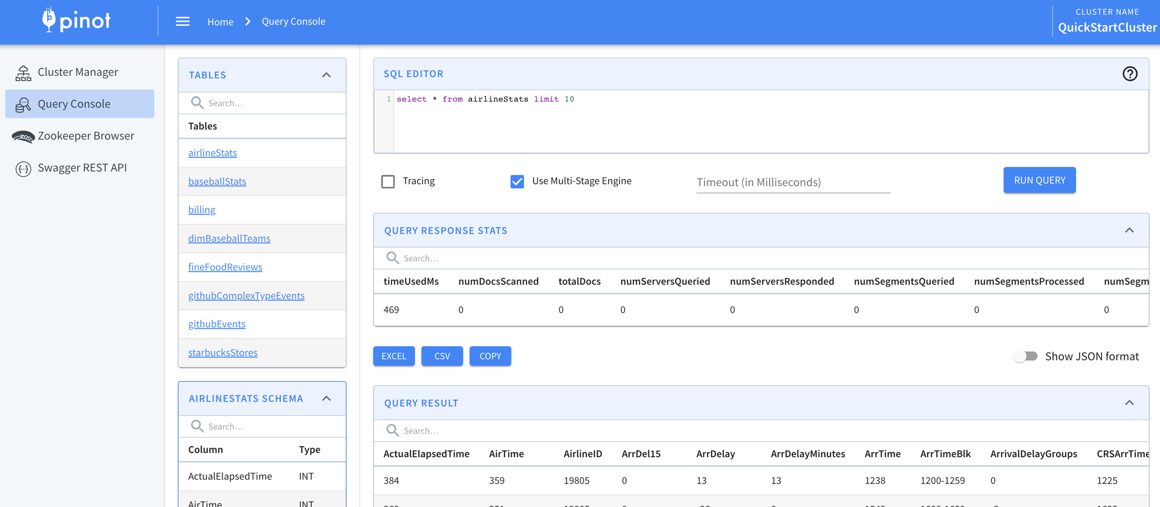
These stats can be seen when using Pinot controller UI by running the query and clicking on the Show JSON format button. Then the whole JSON response will be shown and the multi-stage stats will be in a field called stageStats. Different drivers may provide different ways to see the stats.
broadcast means there are multiple instances of the stream, and all records appear in each instance. This is the most expensive distribution, as it requires sending all the data to all the workers.
Each node in the tree represents an operation that is executed and the tree structure form is similar (but not equal) to the logical plan of the query that can be obtained with the EXPLAIN PLAN command.
As you can see, each operator has a type and the stats carried on the node depend on that type. You can learn more about each operator types and their stats in the Operator Types section.
SELECT playerName, teamName
FROM baseballStats_OFFLINE as playerStats
JOIN dimBaseballTeams_OFFLINE AS teams
ON playerStats.teamID = teams.teamID
LIMIT 10
Groovy Scripts
Pinot allows you to run any function using Apache Groovy scripts. The syntax for executing Groovy script within the query is as follows:
GROOVY('result value metadata json', ''groovy script', arg0, arg1, arg2...)
This function will execute the groovy script using the arguments provided and return the result that matches the provided result value metadata. **** The function requires the following arguments:
Result value metadata json - json string representing result value metadata. Must contain non-null keys resultType and isSingleValue.
Groovy script to execute- groovy script string, which uses arg0, arg1, arg2 etc to refer to the arguments provided within the script
arguments - pinot columns/other transform functions that are arguments to the groovy script
Examples
Add colA and colB and return a single-value INT
groovy( '{"returnType":"INT","isSingleValue":true}', 'arg0 + arg1', colA, colB)\
Find the max element in mvColumn array and return a single-value INT
⚠️ Note that Groovy script doesn't accept Built-In ScalarFunction that's specific to Pinot queries. See the section below for more information.
⚠️Enabling Groovy
Allowing execuatable Groovy in queries can be a security vulnerability. Use caution and be aware of the security risks if you decide to allow groovy. If you would like to enable Groovy in Pinot queries, you can set the following broker config.
pinot.broker.disable.query.groovy=false
If not set, Groovy in queries is disabled by default.
The above configuration applies across the entire Pinot cluster. If you want a table level override to enable/disable Groovy queries, the following property can be set in the query table config.
Scalar Functions
Since the 0.5.0 release, Pinot supports custom functions that return a single output for multiple inputs. Examples of scalar functions can be found in StringFunctions and DateTimeFunctions
Pinot automatically identifies and registers all the functions that have the @ScalarFunction annotation.
Only Java methods are supported.
Adding user defined scalar functions
You can add new scalar functions as follows:
Create a new java project. Make sure you keep the package name as org.apache.pinot.scalar.XXXX
In your java project include the dependency
Annotate your methods with @ScalarFunction annotation. Make sure the method is static and returns only a single value output. The input and output can have one of the following types -
Integer
Long
Double
String
Place the compiled JAR in the /plugins directory in pinot. You will need to restart all Pinot instances if they are already running.
Now, you can use the function in a query as follows:
⚠️ Note that the function name in SQL is the same as the function name in Java. The SQL function name is case-insensitive as well.
EXPLAIN PLAN FOR
select
P_BRAND1, sum(LO_REVENUE)
from ssb_lineorder_1, ssb_part_1
where LO_PARTKEY = P_PARTKEY
and P_CATEGORY = 'MFGR#12'
group by P_BRAND1
If the number of groups of a segment reaches this value, the extra groups will be ignored and the results returned may not be completely accurate. The numGroupsLimitReached property will be set to true in the query response if the value is reached.
Trimming tail groups
After the inner segment groups have been computed, the Pinot query engine optionally trims tail groups. Tail groups are ones that have a lower rank based on the ORDER BY clause used in the query.
This configuration is disabled by default, but can be enabled by configuring the pinot.server.query.executor.min.segment.group.trim.size property.
When segment group trim is enabled, the query engine will trim the tail groups and keep max(<minSegmentGroupTrimSize>, 5 * LIMIT) groups if it gets more groups. Pinot keeps at least 5 * LIMIT groups when trimming tail groups to ensure the accuracy of results.
This value can be overridden on a query by query basis by passing the following option:
Cross segments
Once grouping has been done within a segment, Pinot will merge segment results and trim tail groups and keep max(<minServerGroupTrimSize>, 5 * LIMIT) groups if it gets more groups.
<minServerGroupTrimSize> is set to 5,000 by default and can be adjusted by configuring the pinot.server.query.executor.min.server.group.trim.size property. When setting the configuration to -1, the cross segments trim can be disabled.
This value can be overridden on a query by query basis by passing the following option:
When cross segments trim is enabled, the server will trim the tail groups before sending the results back to the broker. It will also trim the tail groups when the number of groups reaches the <trimThreshold>.
<trimThreshold> is the upper bound of groups allowed in a server for each query to protect servers from running out of memory. To avoid too frequent trimming, the actual trim size is bounded to <trimThreshold> / 2. Combining this with the above equation, the actual trim size for a query is calculated as min(max(<minServerGroupTrimSize>, 5 * LIMIT), <trimThreshold> / 2).
This configuration is set to 1,000,000 by default and can be adjusted by configuring the pinot.server.query.executor.groupby.trim.threshold property.
A higher threshold reduces the amount of trimming done, but consumes more heap memory. If the threshold is set to more than 1,000,000,000, the server will only trim the groups once before returning the results to the broker.
This value can be overridden on a query by query basis by passing the following option:
At Broker
When broker performs the final merge of the groups returned by various servers, there is another level of trimming that takes place. The tail groups are trimmed and max(<minBrokerGroupTrimSize>, 5 * LIMIT) groups are retained.
Default value of <minBrokerGroupTrimSize> is set to 5000. This can be adjusted by configuring pinot.broker.min.group.trim.size property.
GROUP BY behavior
Pinot sets a default LIMIT of 10 if one isn't defined and this applies to GROUP BY queries as well. Therefore, if no limit is specified, Pinot will return 10 groups.
Pinot will trim tail groups based on the ORDER BY clause to reduce the memory footprint and improve the query performance. It keeps at least 5 * LIMIT groups so that the results give good enough approximation in most cases. The configurable min trim size can be used to increase the groups kept to improve the accuracy but has a larger extra memory footprint.
HAVING behavior
If the query has a HAVING clause, it is applied on the merged GROUP BY results that already have the tail groups trimmed. If the HAVING clause is the opposite of the ORDER BY order, groups matching the condition might already be trimmed and not returned. e.g.
Increase min trim size to keep more groups in these cases.
Configuration Parameters
Parameter
Default
Query Override
Description
pinot.server.query.executor.num.groups.limit
The maximum number of groups allowed per segment.
100,000
OPTION(numGroupsLimit=<numGroupsLimit>)
pinot.server.query.executor.min.segment.group.trim.size
The minimum number of groups to keep when trimming groups at the segment level.
pinot.server.query.executor.min.server.group.trim.size
The minimum number of groups to keep when trimming groups at the server level.
Query Options
This document contains all the available query options
Supported Query Options
Key
Description
Default Behavior
timeoutMs
Timeout of the query in milliseconds
Set Query Options
SET statement
After release 0.11.0, query options can be set using the SET statement:
OPTION keyword (deprecated)
Before release 0.11.0, query options can be appended to the query with the OPTION keyword:
REST API
Query options can be specified in API using queryOptions as key and ';' separated key-value pairs.
Alternatively, we can also use the SET keyword in the sql query.
JOINs
Pinot supports JOINs, including left, right, full, semi, anti, lateral, and equi JOINs. Use JOINs to connect two table to generate a unified view, based on a related column between the tables.
Pinot 1.0 introduces support for all JOIN types. JOINs in Pinot significantly reduce query latency and simplify architecture, achieving the best performance currently available for an OLAP database.
Use JOINs to combine two tables (a left and right table) together, based on a related column between the tables, and other join filters. JOINs let you gain more insights from your data.
Supported JOINs types and examples
Inner join
The inner join selects rows that have matching values in both tables.
Syntax:
Example of inner join
Joins a table containing user transactions with a table containing promotions shown to the users, to show the spending for every userID.
Left join
A left join returns all values from the left relation and the matched values from the right table, or appends NULL if there is no match. Also referred to as a left outer join.
Syntax:
Right join
A right join returns all values from the right relation and the matched values from the left relation, or appends NULL if there is no match. It is also referred to as a right outer join.
Syntax:
Full join
A full join returns all values from both relations, appending NULL values on the side that does not have a match. It is also referred to as a full outer join.
Syntax:
Cross join
A cross join returns the Cartesian product of two relations. If no WHERE clause is used along with CROSS JOIN, this produces a result set that is the number of rows in the first table multiplied by the number of rows in the second table. If a WHERE clause is included with CROSS JOIN, it functions like an .
Syntax:
Semi/Anti join
Semi/anti-join returns rows from the first table where no matches are found in the second table. Returns one copy of each row in the first table for which no match is found.
Syntax:
Equi join
An equi join uses an equality operator to match a single or multiple column values of the relative tables.
Syntax:
JOINs optimizations
Pinot JOINs include the following optimizations:
Predicate push-down to individual tables
Indexing and pruning to reduce scanning and speeds up query processing
Smart data layout considerations to minimize data shuffling
Aggregation Functions
Aggregate functions return a single result for a group of rows.
Aggregate functions return a single result for a group of rows. The following table shows supported aggregate functions in Pinot.
Function
Description
Example
Default Value When No Record Selected
Filtering with IdSet
Learn how to write fast queries for looking up IDs in a list of values.
Filtering with IdSet is only supported with the single-stage query engine (v1).
A common use case is filtering on an id field with a list of values. This can be done with the IN clause, but using IN doesn't perform well with large lists of IDs. For large lists of IDs, we recommend using an IdSet.
Explain Plan (Single-Stage)
Query execution within Pinot is modeled as a sequence of operators that are executed in a pipelined manner to produce the final result. The output of the EXPLAIN PLAN statement can be used to see how queries are being run or to further optimize queries.
Introduction
EXPLAN PLAN can be run in two modes: verbose and non-verbose (default) via the use of a query option. To enable verbose mode the query option explainPlanVerbose=true must be passed.
Leaf
Describes the leaf operator in the multi-stage query engine.
The leaf operator is the operator that actually reads the data from the segments. Instead of being just a simple table scan, the leaf operator is a meta-operator that wraps the single-stage query engine and executes all the operators in the leaf stage of the query plan.
Implementation details
The leaf operator is not a relational operator itself but a meta-operator that is able to execute single-stage queries. When servers execute a leaf stage, they compile all operations in the stage but the send operator into the equivalent single-stage query and execute that using a slightly modified version of the single-stage engine.
As a result, leaf stage operators can use all the optimizations and indices that the single-stage engine can use but it also means that there may be slight differences when an operator is executed in a leaf stage compared to when it is executed in an intermediate stage. For example, operations pushed down to the leaf stage may use indexes (see
Join
Describes the hash join relation operator in the multi-stage query engine.
The hash join operator is used to join two relations using a hash join algorithm. It is a binary operator that takes two inputs, the left and right relations, and produces a single output relation.
This is the only join operator in the multi-stage query engine and it is always created as a result of a query that contains a join clause, but can be created by other SQL queries like ones using semi-join.
There are different types of joins that can be performed using the hash join operator. Apache Pinot supports:
Inner join, where only the rows that have a match in both relations are returned.
SELECT *
FROM ...
OPTION(minSegmentGroupTrimSize=<minSegmentGroupTrimSize>)
SELECT *
FROM ...
OPTION(minServerGroupTrimSize=<minServerGroupTrimSize>)
SELECT *
FROM ...
OPTION(groupTrimThreshold=<groupTrimThreshold>)
SELECT SUM(colA)
FROM myTable
GROUP BY colB
HAVING SUM(colA) < 100
ORDER BY SUM(colA) DESC
LIMIT 10
Some functions are only supported in multi-stage and some others only in single-stage.
Type coercion is different. While the single-stage engine always operates with generic types (ie uses doubles when mathematical operations are used), the multi-stage engine tries to keep the types (ie adding two integers will result in an integer).
Blocking nature
One of the slight differences between the leaf and the normal single-stage engine is that the leaf engine tries to be not blocking.
Hints
None
Stats
executionTimeMs
Type: Long
The summation of time spent by all threads executing the operator. This means that the wall time spent in the operation may be smaller that this value if the parallelism is larger than 1.
emittedRows
Type: Long
The number of groups emitted by the operator.
table
Type: String
The name of the table that is scanned. This is the name without the type suffix (so without _REALTIME or _OFFLINE). This is very useful to understand which table is being scanned by this leaf stage in case of complex queries.
numDocsScanned
Type: Long
Similar to the same stat in single-stage queries, this stat indicates the number of rows selected after the filter phase.
If it is very high, that means the selectivity for the query is low and lots of rows need to be processed after the filtering. Consider refining the filter to increase the selectivity of the query.
numEntriesScannedInFilter
Type: Long
Similar to the same stat in single-stage queries, this stat indicates the number of entries (aka scalar values) scanned in the filtering phase of query execution.
Can be larger than the total scanned doc count because of multiple filtering predicates or multi-value entries. Can also be smaller than the total scanned doc count if indexing is used for filtering.
This along with numEntriesScannedPostFilter indicates where most of the time is spent during table scan processing. If this value is high, enabling indexing for affected columns is a way to bring it down. Another option is to partition the data based on the dimension most heavily used in your filter queries.
numEntriesScannedPostFilter
Type: Long
Similar to the same stat in single-stage queries, this stat indicates the number of entries (aka scalar values) scanned after the filtering phase of query execution, ie. aggregation and/or group-by phases. This is equivalent to numDocScanned * number of projected columns.
This along with numEntriesScannedInFilter indicates where most of the time is spent during table scan processing. A high number for this means the selectivity is low (that is, Pinot needs to scan a lot of records to answer the query). If this is high, consider using star-tree index, given a regular index won't improve performance.
numSegmentsQueried
Type: Integer
Similar to the same stat in single-stage queries, this stat indicates the total number of segment queried for a query. May be less than the total number of segments if the broker applies optimizations.
The broker decides how many segments to query on each server, based on broker pruning logic. The server decides how many of these segments to actually look at, based on server pruning logic. After processing segments for a query, fewer may have the matching records.
In general, numSegmentsQueried >= numSegmentsProcessed >= numSegmentsMatched.
numSegmentsProcessed
Type: Integer
Similar to the same stat in single-stage queries, this stat indicates the number of segments processed with at least one document matched in the query response.
The more segments are processed, the more IO has to be done. This is why selective queries where numSegmentsProcessed is close to numSegmentsQueried can be optimized by changing the data distribution.
numSegmentsMatched
Type: Integer
Similar to the same stat in single-stage queries, this stat indicates the number of segment operators used to process segments. Indicates the effectiveness of the pruning logic.
totalDocs
Type: Long
Similar to the same stat in single-stage queries, this stat indicates the number of rows in the table.
numGroupsLimitReached
Type: Boolean
Similar to the same stat in single-stage queries and the same in aggregate operators, this stat indicates if the max group limit has been reached in a group by aggregation operator executed in the leaf stage.
If this boolean is set to true, the query result may not be accurate. The default value for numGroupsLimit is 100k, and should be sufficient for most use cases.
numResizes
Type: Integer
Number of result resizes for queries
resizeTimeMs
Type: Long
Time spent in resizing results for the output. Either because of LIMIT or maximum allowed group by keys or any other criteria.
threadCpuTimeNs
Type: Long
Aggregated thread cpu time in nanoseconds for query processing from servers. This metric is only available if Pinot is configured with pinot.server.instance.enableThreadCpuTimeMeasurement.
systemActivitiesCpuTimeNs
Type: Long
Aggregated system activities cpu time in nanoseconds for query processing (e.g. GC, OS paging etc.) This metric is only available if Pinot is configured with pinot.server.instance.enableThreadCpuTimeMeasurement.
numSegmentsPrunedByServer
Type: Integer
The number of segments pruned by the server, for any reason.
numSegmentsPrunedInvalid
Type: Integer
The number of segments pruned because they are invalid. Segments are invalid when the schema has changed and the segment has not been refreshed.
For example, if a column is added to the schema, the segment will be invalid for queries that use that column until it is refreshed.
numSegmentsPrunedByLimit
Type: Integer
The number of segments pruned because they are not needed for the query due to the limit clause.
Pinot keeps a count of the number of rows returned by each segment. Once it's guaranteed that no more segments need to be read to satisfy the limit clause without breaking semantics, the remaining segments are pruned.
For example, a query like SELECT col1 FROM table2 LIMIT 10 can be pruned for this reason while a query like SELECT col1 FROM table2 ORDER BY col1 DESC LIMIT 10 cannot because Pinot needs to read all segments to guarantee the larger values of col1 are returned.
numSegmentsPrunedByValue
Type: Integer
The number of segments pruned because they are not needed for the query due to a value clause, usually a where.
Pinot keeps the maximum and minimum values of each segment for each column. If the value clause is such that the segment cannot contain any rows that satisfy the clause, the segment is pruned.
numConsumingSegmentsProcessed
Type: Integer
Like numSegmentsProcessed but only for consuming segments.
numConsumingSegmentsMatched
Type: Integer
Like numSegmentsMatched but only for consuming segments.
operatorExecutionTimeMs
Type: Long
The time spent by the operator executing.
operatorExecStartTimeMs
Type: Long
The instant in time when the operator started executing.
Explain attributes
Given that the leaf operator is a meta-operator, it is not actually shown in the explain plan. But the leaf stage is the only operator that can execute table scans, so here we list the attributes that can be found in the explain plan for a table scan
table
Type: String array
Example: table=[[default, userGroups]]
The qualified name of the table that is scanned, which means it also contains the name of the database being used.
Tips and tricks
Try to push as much as possible to the leaf stage
Leaf stage operators can use all the optimizations and indices that the single-stage engine can use. This means that it is usually better to push down as much as possible to the leaf stage.
The engine is smart enough to push down filters and aggregations without breaking semantics, but sometimes there are subtle SQL semantics and what the domain expert writing the query wants to do.
Sometimes things the engine is too paranoid about null handling or the query includes an unnecessary limit clause that prevents the engine from pushing down the filter.
It is recommended to analyze your explain plan to be sure that the engine is able to push down as much logic as you expect.
Enables advanced null handling. See Null value support for more information.(introduced in 0.11.0)
false (disabled)
explainPlanVerbose
Return verbose result for EXPLAIN query (introduced in 0.11.0)
false (not verbose)
useMultistageEngine
Use multi-stage engine to execute the query (introduced in 0.11.0)
false (use single-stage engine)
maxExecutionThreads
Maximum threads to use to execute the query. Useful to limit the resource usage for expensive queries
Half of the CPU cores for non-group-by queries; all CPU cores for group-by queries
numReplicaGroupsToQuery
When replica-group based routing is enabled, use it to query multiple replica-groups (introduced in 0.11.0)
1 (only query servers within the same replica-group)
minSegmentGroupTrimSize
Minimum groups to keep when trimming groups at the segment level for group-by queries. See Configuration Parameters
Server level config
minServerGroupTrimSize
Minimum groups to keep when trimming groups at the server level for group-by queries. See Configuration Parameters
Server level config
skipIndexes
Which indexes to skip usage of (i.e. scan instead), per-column. This is useful for side-by-side comparison/debugging. There can be cases where the use of an index is actually more expensive than performing a scan of the docs which match other filters. One such example could be a low-selectivity inverted index used in conjunction with another highly selective filter.
Config can be specified using url parameter format: skipIndexes='col1=inverted,range&col2=inverted'
Possible index types to skip are: sorted, range, inverted, H3. To find out which indexes are used to resolve a given query, use the EXPLAIN query.
Configure maximum rows allowed in join hash-table creation phase
default value read from cluster config
if not set, the default will be
2^20 (1024*1024)
inPredicatePreSorted
(Only apply to STRING columns) Indicates that the values in the IN clause is already sorted, so that Pinot doesn't need to sort them again at query time
false (values in IN predicate is not pre-sorted)
inPredicateLookupAlgorithm
(Only apply to STRING columns) The algorithm to use to look up the dictionary ids for the IN clause values.
DIVIDE_BINARY_SEARCH: Sort the IN clause values and do binary search on both dictionary and IN clause values at same time to reduce the value lookups
SCAN: Sort the IN clause values and scan both dictionary and IN clause values to get the matching dictionary ids
PLAIN_BINARY_SEARCH: Do not sort the IN clause values, but directly binary search each IN clause value in the dictionary
DIVIDE_BINARY_SEARCH
maxServerResponseSizeBytes
Long value config indicating the maximum length of the serialized response per server for a query.
Long value config indicating the maximum serialized response size across all servers for a query. This value is equally divided across all servers processing the query.
This function returns a base 64 encoded IdSet of the values for a single column. The IdSet implementation used depends on the column data type:
INT - RoaringBitmap unless sizeThresholdInBytes is exceeded, in which case Bloom Filter.
LONG - Roaring64NavigableMap unless sizeThresholdInBytes is exceeded, in which case Bloom Filter.
Other types - Bloom Filter
The following parameters are used to configure the Bloom Filter:
expectedInsertions - Number of expected insertions for the BloomFilter, must be positive
fpp - False positive probability to use for the BloomFilter. Must be positive and less than 1.0.
Note that when a Bloom Filter is used, the filter results are approximate - you can get false-positive results (for membership in the set), leading to potentially unexpected results.
IN_ID_SET
IN_ID_SET(columnName, base64EncodedIdSet)
This function returns 1 if a column contains a value specified in the IdSet and 0 if it does not.
IN_SUBQUERY
IN_SUBQUERY(columnName, subQuery)
This function generates an IdSet from a subquery and then filters ids based on that IdSet on a Pinot broker.
IN__PARTITIONED__SUBQUERY
IN_PARTITIONED_SUBQUERY(columnName, subQuery)
This function generates an IdSet from a subquery and then filters ids based on that IdSet on a Pinot server.
This function works best when the data is partitioned by the id column and each server contains all the data for a partition. The generated IdSet for the subquery will be smaller as it will only contain the ids for the partitions served by the server. This will give better performance.
The query passed to IN_SUBQUERY can be run on any table - they aren't restricted to the table used in the parent query.
The query passed to IN__PARTITIONED__SUBQUERY must be run on the same table as the parent query.
Examples
Create IdSet
You can create an IdSet of the values in the yearID column by running the following:
We can use the IN_ID_SET function to filter a query based on an IdSet. To return rows for _yearID_s in the IdSet, run the following:
Filter by values not in IdSet
To return rows for _yearID_s not in the IdSet, run the following:
Filter on broker
To filter rows for _yearID_s in the IdSet on a Pinot Broker, run the following query:
To filter rows for _yearID_s not in the IdSet on a Pinot Broker, run the following query:
Filter on server
To filter rows for _yearID_s in the IdSet on a Pinot Server, run the following query:
To filter rows for _yearID_s not in the IdSet on a Pinot Server, run the following query:
In the non-verbose EXPLAIN PLAN output above, the Operator column describes the operator that Pinot will run where as, the Operator_Id and Parent_Id columns show the parent-child relationship between operators.
This parent-child relationship shows the order in which operators execute. For example, FILTER_MATCH_ENTIRE_SEGMENT will execute before and pass its output to PROJECT. Similarly, PROJECT will execute before and pass its output to TRANSFORM_PASSTHROUGH operator and so on.
Although the EXPLAIN PLAN query produces tabular output, in this document, we show a tree representation of the EXPLAIN PLAN output so that parent-child relationship between operators are easy to see and user can visualize the bottom-up flow of data in the operator tree execution.
Note a special node with the Operator_Id and Parent_Id called PLAN_START(numSegmentsForThisPlan:1). This node indicates the number of segments which match a given plan. The EXPLAIN PLAN query can be run with the verbose mode enabled using the query option explainPlanVerbose=true which will show the varying deduplicated query plans across all segments across all servers.
EXPLAIN PLAN output should only be used for informational purposes because it is likely to change from version to version as Pinot is further developed and enhanced. Pinot uses a "Scatter Gather" approach to query evaluation (see Pinot Architecture for more details). At the Broker, an incoming query is split into several server-level queries for each backend server to evaluate. At each Server, the query is further split into segment-level queries that are evaluated against each segment on the server. The results of segment queries are combined and sent to the Broker. The Broker in turn combines the results from all the Servers and sends the final results back to the user. Note that if the EXPLAIN PLAN query runs without the verbose mode enabled, a single plan will be returned (the heuristic used is to return the deepest plan tree) and this may not be an accurate representation of all plans across all segments. Different segments may execute the plan in a slightly different way.
Reading the EXPLAIN PLAN output from bottom to top will show how data flows from a table to query results. In the example shown above, the FILTER_MATCH_ENTIRE_SEGMENT operator shows that all 977889 records of the segment matched the query. The DOC_ID_SET over the filter operator gets the set of document IDs matching the filter operator. The PROJECT operator over the DOC_ID_SET operator pulls only those columns that were referenced in the query. The TRANSFORM_PASSTHROUGH operator just passes the column data from PROJECT operator to the SELECT operator. At SELECT, the query has been successfully evaluated against one segment. Results from different data segments are then combined (COMBINE_SELECT) and sent to the Broker. The Broker combines and reduces the results from different servers (BROKER_REDUCE) into a final result that is sent to the user. The PLAN_START(numSegmentsForThisPlan:1) indicates that a single segment matched this query plan. If verbose mode is enabled many plans can be returned and each will contain a node indicating the number of matched segments.
The rest of this document illustrates the EXPLAIN PLAN output with examples and describe the operators that show up in the output of the EXPLAIN PLAN.
EXPLAIN PLAN using verbose mode for a query that evaluates filters with and without index
Since verbose mode is enabled, the EXPLAIN PLAN output returns two plans matching one segment each (assuming 2 segments for this table). The first EXPLAIN PLAN output above shows that Pinot used an inverted index to evaluate the predicate "playerID = 'aardsda01'" (FILTER_INVERTED_INDEX). The result was then fully scanned (FILTER_FULL_SCAN) to evaluate the second predicate "playerName = 'David Allan'". Note that the two predicates are being combined using AND in the query; hence, only the data that satsified the first predicate needs to be scanned for evaluating the second predicate. However, if the predicates were being combined using OR, the query would run very slowly because the entire "playerName" column would need to be scanned from top to bottom to look for values satisfying the second predicate. To improve query efficiency in such cases, one should consider indexing the "playerName" column as well. The second plan output shows a FILTER_EMPTY indicating that no matching documents were found for one segment.
EXPLAIN PLAN ON GROUP BY QUERY
The EXPLAIN PLAN output above shows how GROUP BY queries are evaluated in Pinot. GROUP BY results are created on the server (AGGREGATE_GROUPBY_ORDERBY) for each segment on the server. The server then combines segment-level GROUP BY results (COMBINE_GROUPBY_ORDERBY) and sends the combined result to the Broker. The Broker combines GROUP BY result from all the servers to produce the final result which is send to the user. Note that the COMBINE_SELECT operator from the previous query was not used here, instead a different COMBINE_GROUPBY_ORDERBY operator was used. Depending upon the type of query different combine operators such as COMBINE_DISTINCT and COMBINE_ORDERBY etc may be seen.
EXPLAIN PLAN OPERATORS
The root operator of the EXPLAIN PLAN output is BROKER_REDUCE. BROKER_REDUCE indicates that Broker is processing and combining server results into final result that is sent back to the user. BROKER_REDUCE has a COMBINE operator as its child. Combine operator combines the results of query evaluation from each segment on the server and sends the combined result to the Broker. There are several combine operators (COMBINE_GROUPBY_ORDERBY, COMBINE_DISTINCT, COMBINE_AGGREGATE, etc.) that run depending upon the operations being performed by the query. Under the Combine operator, either a Select (SELECT, SELECT_ORDERBY, etc.) or an Aggregate (AGGREGATE, AGGREGATE_GROUPBY_ORDERBY, etc.) can appear. Aggreate operator is present when query performs aggregation (count(*), min, max, etc.); otherwise, a Select operator is present. If the query performs scalar transformations (Addition, Multiplication, Concat, etc.), then one would see TRANSFORM operator appear under the SELECT operator. Often a TRANSFORM_PASSTHROUGH operator is present instead of the TRANSFORM operator. TRANSFORM_PASSTHROUGH just passes results from operators that appear lower in the operator execution heirarchy to the SELECT operator. DOC_ID_SET operator usually appear above FILTER operators and indicate that a list of matching document IDs are assessed. FILTER operators usually appear at the bottom of the operator heirarchy and show index use. For example, the presence of FILTER_FULL_SCAN indicates that index was not used (and hence the query is likely to run relatively slow). However, if the query used an index one of the indexed filter operators (FILTER_SORTED_INDEX, FILTER_RANGE_INDEX, FILTER_INVERTED_INDEX, FILTER_JSON_INDEX, etc.) will show up.
Left join, where all the rows from the left relation are returned. The ones that have a match with the right relation are returned with the columns from the right relation, and the ones that do not have a match are returned with null values for the columns from the right relation.
Right join, like the left join but returning all the rows from the right relation, with the columns from the left relation filled with null values for the rows that do not have a match.
Full outer join, where all the rows from both relations are returned. If a row from any relation does not have a match in the other relation, the columns from the other relation are filled with null values.
Semi-join, where only the rows from the left relation that have a match in the right relation are returned. This is useful to filter the rows from the left relation based on the existence of a match in the right relation.
Anti-join, where only the rows from the left relation that do not have a match in the right relation are returned.
Implementation details
The hash join operator is one of the new operators introduced in the multi-stage query engine. The current implementation assumes that the right input relation is the smaller one, so it consumes this input first building a hash table that is then probed with the left input relation.
Future optimizations may include advanced heuristics to decide which input relation to consume first, but in the current implementation, it is important to specify the smaller relation as the right input.
Although the whole multi-stage query engine is designed to be able to process the data in memory, the multi-stage query engine uses the ability to execute each stage in different workers (explained in understanding stages) to be able to process the data that may not fit in the memory of a single node. Specifically, each worker processes a subset of the data. Inputs are by default partitioned by the join keys and each worker process one partition of the data.
This means that data usually needs to be shuffled between workers, which is done by the engine using a mailbox system. The engine tries to minimize the amount of data that needs to be shuffled by partitioning the data, but some techniques can be used to reduce the amount of data that needs to be shuffled, like using co-located joins.
Blocking nature
The hash join operator is a blocking operator. It needs to consume all the input data (from both inputs) before emitting the result.
Maximum number of groups
Even using partitioning, the amount of data that needs to be stored in memory can be high, so the engine tries to protect itself from running out of memory by limiting the number of groups that can be created by the join keys.
The join_overflow_mode hint can be used to control the behavior of the engine when the number of groups exceeds the limit. This limit can be defined using the max_rows_in_join hint. By default, this limit is slightly above 1 million groups and the default join overflow mode is THROW, which means that the query will fail if the number of groups exceeds the limit.
Hints
join_overflow_mode
Type: String
Default: THROW
Defines the behavior of the engine when the number of groups exceeds the limit defined by the max_rows_in_join hint. The possible values are:
THROW: The query will fail if the number of groups exceeds the limit.
BREAK: The engine will stop processing the join and return the results that have been computed so far. In this case the stat maxRowsInJoinReached will be true.
max_rows_in_join
Type: Integer
Default: 1.048.576
The maximum number of groups that can be created by the join keys. What happens when this limit is reached is defined by the join_overflow_mode hint.
Take care when increasing this limit. If the number of groups is too high, the amount of memory used by the engine can be very high, which can lead to very large GC pauses and even out of memory errors.
Stats
executionTimeMs
Type: Long
The summation of time spent by all threads executing the operator. This means that the wall time spent in the operation may be smaller that this value if the parallelism is larger than 1.
emittedRows
Type: Long
The number of groups emitted by the operator. Joins can emit more rows than the input relations, so this value can be higher than the number of rows in the input. Remember that the number of groups is limited by the max_rows_in_join hint and a large number of groups can lead to high memory usage and long GC pauses, which can affect the performance of the whole system.
maxRowsInJoinReached
Type: Boolean
This stat is set to true when the number of groups exceeds the limit defined by the max_rows_in_join hint.
Notice that by default the engine will throw an exception when this happens in which case no stat will be emitted. Therefore this stat is only emitted when the join_overflow_mode hint is set to BREAK.
timeBuildingHashTableMs
Type: Long
The time spent building the hash table used to probe the join keys, in milliseconds.
A large number here can indicate that the right relation is too large or the right relation is taking too long to be processed.
Explain attributes
The hash join operator is represented in the explain plan as a LogicalJoin explain node.
condition
Type: Expression
The condition that is being applied to the rows to join the relations. The expression may use indexed columns ($0, $1, etc), functions and literals. The indexed columns are always 0-based.
For example, the following explain plan:
Is saying that the join condition is that the column with index 0 in the left relation is equal to the column with index 1 in the right relation. Given the rest of the explain plan, we can see that the column with index 0 userUUID column in the userAttributes table and the column with index 1 is the userUUID column in the userGroups table.
joinType
Type: String
The type of join that is being performed. The possible values are: inner, left, right, full, semi and anti, as explained in Implementation details.
Tips and tricks
The order of input relations matter
Apache Pinot does not use table stats to determine the best order to consume the input relations. Instead, it assumes that the right input relation is the smaller one. That relation will always be fully consumed to build a hash table and sometimes it will be broadcasted to all workers. This means that it is important to specify the smaller relation as the right input.
Remember that left and right are relative to the order of the tables in the SQL query. It is less expensive to do a join between a large table and a small table than the other way around.
For example, this query:
is more efficient than:
pinot.query.join.max.rows
SET key1 = 'value1';
SET key2 = 123;
SELECT * FROM myTable
SELECT * FROM myTable OPTION(key1=value1, key2=123)
SELECT * FROM myTable OPTION(key1=value1) OPTION(key2=123)
SELECT * FROM myTable OPTION(timeoutMs=30000)
curl -X POST 'http://localhost:9000/sql' \
-d '{
"sql": "SELECT * FROM myTable",
"trace": false,
"queryOptions":"key1=value1;key2=123"
}'
curl -X POST 'http://localhost:8099/query/sql' \
-d '{
"sql": "SELECT * FROM myTable;",
"trace": false,
"queryOptions":"key1=value1;key2=123"
}'
SELECT myTable.column1,myTable.column2,myOtherTable.column1,....
FROM mytable INNER JOIN table2
ON table1.matching_column = myOtherTable.matching_column;
SELECT
p.userID, t.spending_val
FROM promotion AS p JOIN transaction AS t
ON p.userID = t.userID
WHERE
p.promotion_val > 10
AND t.transaction_type IN ('CASH', 'CREDIT')
AND t.transaction_epoch >= p.promotion_start_epoch
AND t.transaction_epoch < p.promotion_end_epoch
SELECT myTable.column1,table1.column2,myOtherTable.column1,....
FROM myTable LEFT JOIN myOtherTable
ON myTable.matching_column = myOtherTable.matching_column;
SELECT table1.column1,table1.column2,table2.column1,....
FROM table1
RIGHT JOIN table2
ON table1.matching_column = table2.matching_column;
SELECT table1.column1,table1.column2,table2.column1,....
FROM table1
FULL JOIN table2
ON table1.matching_column = table2.matching_column;
SELECT *
FROM table1
CROSS JOIN table2;
SELECT myTable.column1, myOtherTable.column1
FROM myOtherTable
WHERE NOT EXISTS [ join_criteria ]
SELECT *
FROM table1
JOIN table2
[ON (join_condition)]
OR
SELECT column_list
FROM table1, table2....
WHERE table1.column_name =
table2.column_name;
SELECT ID_SET(yearID)
FROM baseballStats
WHERE teamID = 'WS1'
SELECT ID_SET(playerName, 'expectedInsertions=10')
FROM baseballStats
WHERE teamID = 'WS1'
SELECT ID_SET(playerName, 'expectedInsertions=100')
FROM baseballStats
WHERE teamID = 'WS1'
SELECT ID_SET(playerName, 'expectedInsertions=100;fpp=0.01')
FROM baseballStats
WHERE teamID = 'WS1'
SELECT yearID, count(*)
FROM baseballStats
WHERE IN_ID_SET(
yearID,
'ATowAAABAAAAAAA7ABAAAABtB24HbwdwB3EHcgdzB3QHdQd2B3cHeAd5B3oHewd8B30Hfgd/B4AHgQeCB4MHhAeFB4YHhweIB4kHigeLB4wHjQeOB48HkAeRB5IHkweUB5UHlgeXB5gHmQeaB5sHnAedB54HnwegB6EHogejB6QHpQemB6cHqAc='
) = 1
GROUP BY yearID
SELECT yearID, count(*)
FROM baseballStats
WHERE IN_ID_SET(
yearID,
'ATowAAABAAAAAAA7ABAAAABtB24HbwdwB3EHcgdzB3QHdQd2B3cHeAd5B3oHewd8B30Hfgd/B4AHgQeCB4MHhAeFB4YHhweIB4kHigeLB4wHjQeOB48HkAeRB5IHkweUB5UHlgeXB5gHmQeaB5sHnAedB54HnwegB6EHogejB6QHpQemB6cHqAc='
) = 0
GROUP BY yearID
SELECT yearID, count(*)
FROM baseballStats
WHERE IN_SUBQUERY(
yearID,
'SELECT ID_SET(yearID) FROM baseballStats WHERE teamID = ''WS1'''
) = 1
GROUP BY yearID
SELECT yearID, count(*)
FROM baseballStats
WHERE IN_SUBQUERY(
yearID,
'SELECT ID_SET(yearID) FROM baseballStats WHERE teamID = ''WS1'''
) = 0
GROUP BY yearID
SELECT yearID, count(*)
FROM baseballStats
WHERE IN_PARTITIONED_SUBQUERY(
yearID,
'SELECT ID_SET(yearID) FROM baseballStats WHERE teamID = ''WS1'''
) = 1
GROUP BY yearID
SELECT yearID, count(*)
FROM baseballStats
WHERE IN_PARTITIONED_SUBQUERY(
yearID,
'SELECT ID_SET(yearID) FROM baseballStats WHERE teamID = ''WS1'''
) = 0
GROUP BY yearID
Returns the average of the values for a numeric column as Double
AVG(playerScore)
Double.NEGATIVE_INFINITY
Returns the most frequent value of a numeric column as Double. When multiple modes are present it gives the minimum of all the modes. This behavior can be overridden to get the maximum or the average mode.
MODE(playerScore)
MODE(playerScore, 'MIN')
MODE(playerScore, 'MAX')
MODE(playerScore, 'AVG')
Double.NEGATIVE_INFINITY
Returns the max - min value for a numeric column as Double
MINMAXRANGE(playerScore)
Double.NEGATIVE_INFINITY
Returns the Nth percentile of the values for a numeric column as Double. N is a decimal number between 0 and 100 inclusive.
Returns the Nth percentile of the values for a numeric column using as Long
PERCENTILEEST(playerScore, 50)
PERCENTILEEST(playerScore, 99.9)
Long.MIN_VALUE
Returns the Nth percentile of the values for a numeric column using as Double
PERCENTILETDIGEST(playerScore, 50)
PERCENTILETDIGEST(playerScore, 99.9)
Double.NaN
Returns the Nth percentile (using compression factor of CF) of the values for a numeric column using as Double
PERCENTILETDIGEST(playerScore, 50, 1000)
PERCENTILETDIGEST(playerScore, 99.9, 500)
Double.NaN
PERCENTILESMARTTDIGEST
Returns the Nth percentile of the values for a numeric column as Double. When there are too many values, automatically switch to approximate percentile using TDigest. The switch threshold (100_000 by default) and compression (100 by default) for the TDigest can be configured via the optional second argument.
Returns the count of distinct values of a column as Integer
DISTINCTCOUNT(playerName)
0
Returns the count of distinct values of a column as Integer. This function is accurate for INT column, but approximate for other cases where hash codes are used in distinct counting and there may be hash collisions.
DISTINCTCOUNTBITMAP(playerName)
0
Returns an approximate distinct count using HyperLogLog asLong. It also takes an optional second argument to configure the log2m for the HyperLogLog.
DISTINCTCOUNTHLL(playerName, 12)
0
Returns HyperLogLog response serialized as String. The serialized HLL can be converted back into an HLL and then aggregated with other HLLs. A common use case may be to merge HLL responses from different Pinot tables, or to allow aggregation after client-side batching.
DISTINCTCOUNTRAWHLL(playerName)
0
Returns an approximate distinct count using HyperLogLogPlus asLong. It also takes an optional second and third arguments to configure the p and sp for the HyperLogLogPlus.
DISTINCTCOUNTHLLPLUS(playerName)
0
Returns HyperLogLogPlus response serialized as String. The serialized HLLPlus can be converted back into an HLLPlus and then aggregated with other HLLPluses. A common use case may be to merge HLLPlus responses from different Pinot tables, or to allow aggregation after client-side batching.
DISTINCTCOUNTRAWHLLPLUS(playerName)
0
DISTINCTCOUNTSMARTHLL
Returns the count of distinct values of a column as Integer. When there are too many distinct values, automatically switch to approximate distinct count using HyperLogLog. The switch threshold (100_000 by default) and log2m (12 by default) for the HyperLogLog can be configured via the optional second argument.
Returns the count of distinct values of a column as Long when the column is pre-partitioned for each segment, where there is no common value within different segments. This function calculates the exact count of distinct values within the segment, then simply sums up the results from different segments to get the final result.
SEGMENTPARTITIONEDDISTINCTCOUNT(playerName)
0
See
0
Get the last value of dataColumn where the timeColumn is used to define the time of dataColumn and the dataType specifies the type of dataColumn, which can be BOOLEAN, INT, LONG, FLOAT, DOUBLE, STRING
Get the first value of dataColumn where the timeColumn is used to define the time of dataColumn and the dataType specifies the type of dataColumn, which can be BOOLEAN, INT, LONG, FLOAT, DOUBLE, STRING
FASTHLL stores serialized HyperLogLog in String format, which performs worse than DISTINCTCOUNTHLL, which supports serialized HyperLogLog in BYTES (byte array) format
FASTHLL(playerName)
Multi-value column functions
The following aggregation functions can be used for multi-value columns
Function
Returns the count of a multi-value column as Long
Returns the minimum value of a numeric multi-value column as Double
Returns the maximum value of a numeric multi-value column as Double
Returns the sum of the values for a numeric multi-value column as Double
Returns the average of the values for a numeric multi-value column as Double
Returns the max - min value for a numeric multi-value column as Double
Returns the Nth percentile of the values for a numeric multi-value column as Double
Returns the Nth percentile using as Long
Returns the Nth percentile using as Double
Returns the Nth percentile (using compression factor CF) using as Double
Returns the count of distinct values for a multi-value column as Integer
FILTER Clause in aggregation
Pinot supports FILTER clause in aggregation queries as follows:
In the query above, COL1 is aggregated only for rows where COL2 > 300 and COL3 > 50 . Similarly, COL2 is aggregated where COL2 < 50 and COL3 > 50.
With NULL Value Support enabled, this allows to filter out the null values while performing aggregation as follows:
In the above query, COL1 is aggregated only for the non-null values. Without NULL value support, we would have to filter using the default null value.
Deprecated functions:
Function
Description
Example
FASTHLLMV (Deprecated)
stores serialized HyperLogLog in String format, which performs worse than DISTINCTCOUNTHLL, which supports serialized HyperLogLog in BYTES (byte array) format
Cardinality estimation is a classic problem. Pinot solves it with multiple ways each of which has a trade-off between accuracy and latency.
Exact Results
Functions:
SELECT SUM(COL1) FILTER (WHERE COL2 > 300),
AVG(COL2) FILTER (WHERE COL2 < 50)
FROM MyTable WHERE COL3 > 50
SELECT SUM(COL1) FILTER (WHERE COL1 IS NOT NULL)
FROM MyTable WHERE COL3 > 50
DISTINCTCOUNTBITMAPMV
Returns the count of distinct values for a multi-value column as Integer. This function is accurate for INT or dictionary encoded column, but approximate for other cases where hash codes are used in distinct counting and there may be hash collision.
DISTINCTCOUNTHLLMV
Returns an approximate distinct count using HyperLogLog as Long
DISTINCTCOUNTRAWHLLMV
Returns HyperLogLog response serialized as string. The serialized HLL can be converted back into an HLL and then aggregated with other HLLs. A common use case may be to merge HLL responses from different Pinot tables, or to allow aggregation after client-side batching.
DISTINCTCOUNTHLLPLUSMV
Returns an approximate distinct count using HyperLogLogPlus as Long
DISTINCTCOUNTRAWHLLPLUSMV
Returns HyperLogLogPlus response serialized as string. The serialized HLLPlus can be converted back into an HLLPlus and then aggregated with other HLLPluses. A common use case may be to merge HLLPlus responses from different Pinot tables, or to allow aggregation after client-side batching.
Returns accurate count for all unique values in a column.
The underlying implementation is using a IntOpenHashSet in library: it.unimi.dsi:fastutil:8.2.3 to hold all the unique values.
Approximate Results
It usually takes a lot of resources and time to compute exact results for unique counting on large datasets. In some circumstances, we can tolerate a certain error rate, in which case we can use approximation functions to tackle this problem.
HyperLogLog
HyperLogLog is an approximation algorithm for unique counting. It uses fixed number of bits to estimate the cardinality of given data set.
Pinot leverages HyperLogLog Class in library com.clearspring.analytics:stream:2.7.0as the data structure to hold intermediate results.
Functions:
DistinctCountHLL(x)_ -> LONG_
For column type INT/LONG/FLOAT/DOUBLE/STRING, Pinot treats each value as an individual entry to add into HyperLogLog Object, and then computes the approximation by calling method _cardinality().
For column type BYTES, Pinot treats each value as a serialized HyperLogLog Object with pre-aggregated values inside. The bytes value is generated by org.apache.pinot.core.common.ObjectSerDeUtils.HYPER_LOG_LOG_SER_DE.serialize(hyperLogLog).
All deserialized HyperLogLog object will be merged into one then calling method _cardinality() to get the approximated unique count._
HyperLogLogPlusPlus
The HyperLogLog++ algorithm proposes several improvements in the HyperLogLog algorithm to reduce memory requirements and increase accuracy in some ranges of cardinalities.
64-bit hash function is used instead of the 32 bits used in the original paper. This reduces the hash collisions for large cardinalities allowing to remove the large range correction.
Some bias is found for small cardinalities when switching from linear counting to the HLL counting. An empirical bias correction is proposed to mitigate the problem.
A sparse representation of the registers is implemented to reduce memory requirements for small cardinalities, which can be later transformed to a dense representation if the cardinality grows.
Pinot leverages HyperLogLogPlus Class in library com.clearspring.analytics:stream:2.7.0as the data structure to hold intermediate results.
For column type INT/LONG/FLOAT/DOUBLE/STRING , Pinot treats each value as an individual entry to add into HyperLogLogPlus Object, then compute the approximation by calling method _cardinality().
For column type BYTES, Pinot treats each value as a serialized HyperLogLogPlus Object with pre-aggregated values inside. The bytes value is generated by org.apache.pinot.core.common.ObjectSerDeUtils.HYPER_LOG_LOG_PLUS_SER_DE.serialize(hyperLogLogPlus).
All deserialized HyperLogLogPlus object will be merged into one then calling method _cardinality() to get the approximated unique count._
Theta Sketches
The Theta Sketch framework enables set operations over a stream of data, and can also be used for cardinality estimation. Pinot leverages the Sketch Class and its extensions from the library org.apache.datasketches:datasketches-java:4.2.0 to perform distinct counting as well as evaluating set operations.
Functions:
DistinctCountThetaSketch(<thetaSketchColumn>, <thetaSketchParams>, predicate1, predicate2..., postAggregationExpressionToEvaluate**) **-> LONG
thetaSketchColumn (required): Name of the column to aggregate on.
thetaSketchParams (required): Parameters for constructing the intermediate theta-sketches. Currently, the only supported parameter is nominalEntries.
predicates (optional)_: _ These are individual predicates of form lhs <op> rhs which are applied on rows selected by the where clause. During intermediate sketch aggregation, sketches from the thetaSketchColumn that satisfies these predicates are unionized individually. For example, all filtered rows that match country=USA are unionized into a single sketch. Complex predicates that are created by combining (AND/OR) of individual predicates is supported.
postAggregationExpressionToEvaluate (required): The set operation to perform on the individual intermediate sketches for each of the predicates. Currently supported operations are SET_DIFF, SET_UNION, SET_INTERSECT , where DIFF requires two arguments and the UNION/INTERSECT allow more than two arguments.
In the example query below, the where clause is responsible for identifying the matching rows. Note, the where clause can be completely independent of the postAggregationExpression. Once matching rows are identified, each server unionizes all the sketches that match the individual predicates, i.e. country='USA' , device='mobile' in this case. Once the broker receives the intermediate sketches for each of these individual predicates from all servers, it performs the final aggregation by evaluating the postAggregationExpression and returns the final cardinality of the resulting sketch.
This is the same as the previous function, except it returns the byte serialized sketch instead of the cardinality sketch. Since Pinot returns responses as JSON strings, bytes are returned as hex encoded strings. The hex encoded string can be deserialized into sketch by using the library org.apache.commons.codec.binaryas Hex.decodeHex(stringValue.toCharArray()).
Tuple Sketches
The Tuple Sketch is an extension of the Theta Sketch. Tuple sketches store an additional summary value with each retained entry which makes the sketch ideal for summarizing attributes such as impressions or clicks. Tuple sketches are interoperable with the Theta Sketch and enable set operations over a stream of data, and can also be used for cardinality estimation.
Functions:
avgValueIntegerSumTupleSketch(<tupleSketchColumn>, <tupleSketchLgK>**) -> Long
tupleSketchColumn (required): Name of the column to aggregate on.
tupleSketchLgK (optional): lgK which is the the log2 of K, which controls both the size and accuracy of the sketch.
This function can be used to combine the summary values from the random sample stored within the Tuple sketch and formulate an estimate for an average that applies to the entire dataset. The average should be interpreted as applying to each key tracked by the sketch and is rounded to the nearest whole number.
distinctCountTupleSketch(<tupleSketchColumn>, <tupleSketchLgK>**) -> LONG
tupleSketchColumn (required): Name of the column to aggregate on.
tupleSketchLgK (optional): lgK which is the the log2 of K, which controls both the size and accuracy of the sketch.
This returns the cardinality estimate for a column where the values are already encoded as Tuple sketches, stored as BYTES.
This is the same as the previous function, except it returns the byte serialized sketch instead of the cardinality sketch. Since Pinot returns responses as JSON strings, bytes are returned as hex encoded strings. The hex encoded string can be deserialized into sketch by using the library org.apache.commons.codec.binaryas Hex.decodeHex(stringValue.toCharArray()).
sumValuesIntegerSumTupleSketch(<tupleSketchColumn>, <tupleSketchLgK>**) -> Long
tupleSketchColumn (required): Name of the column to aggregate on.
tupleSketchLgK (optional): lgK which is the the log2 of K, which controls both the size and accuracy of the sketch.
This function can be used to combine the summary values (using sum) from the random sample stored within the Tuple sketch and formulate an estimate that applies to the entire dataset. See avgValueIntegerSumTupleSketch for extracting an average for integer summaries. If other merging options are required, it is best to extract the raw sketches directly or to implement a new Pinot aggregation function to support these.
Compressed Probability Counting (CPC) Sketches
The Compressed Probability Counting(CPC) Sketch enables extremely space-efficient cardinality estimation. The stored CPC sketch can consume about 40% less space than an HLL sketch of comparable accuracy. Pinot can aggregate multiple existing CPC sketches together to get a total distinct count or estimated directly from raw values.
Functions:
distinctCountCpcSketch(<cpcSketchColumn>, <cpcSketchLgK>**) -> Long
cpcSketchColumn (required): Name of the column to aggregate on.
cpcSketchLgK (optional): lgK which is the the log2 of K, which controls both the size and accuracy of the sketch.
This returns the cardinality estimate for a column.
cpcSketchColumn (required): Name of the column to aggregate on.
cpcSketchLgK (optional): lgK which is the the log2 of K, which controls both the size and accuracy of the sketch.
This is the same as the previous function, except it returns the byte serialized sketch instead of the cardinality sketch. Since Pinot returns responses as JSON strings, bytes are returned as hex encoded strings. The hex encoded string can be deserialized into sketch by using the library org.apache.commons.codec.binaryas Hex.decodeHex(stringValue.toCharArray()).
UltraLogLog (ULL) Sketches
The UltraLogLog Sketch from Dynatrace is a variant of HyperLogLog and is used for approximate distinct counts. The UltraLogLog sketch shares many of the same properties of a typical HyperLogLog sketch but requires less space and also provides a simpler and faster estimator.
Pinot uses an production-ready Java implementation available in Hash4j available under the Apache license.
Functions:
distinctCountULL(<ullSketchColumn>, <ullSketchPrecision>**) -> Long
ullSketchColumn (required): Name of the column to aggregate on.
ullSketchPrecision (optional): p which is the precision parameter, which controls both the size and accuracy of the sketch.
This returns the cardinality estimate for a column.
ullSketchColumn (required): Name of the column to aggregate on.
ullSketchPrecision (optional): p which is the precision parameter, which controls both the size and accuracy of the sketch.
This is the same as the previous function, except it returns the byte serialized sketch instead of the cardinality sketch. Since Pinot returns responses as JSON strings, bytes are returned as hex encoded strings. The hex encoded string can be deserialized into sketch by using the library org.apache.commons.codec.binaryas Hex.decodeHex(stringValue.toCharArray()).
select distinctCountThetaSketch(
sketchCol,
'nominalEntries=1024',
'country'=''USA'' AND 'state'=''CA'', 'device'=''mobile'', 'SET_INTERSECT($1, $2)'
)
from table
where country = 'USA' or device = 'mobile...'
Lookup UDF Join
For more information about using JOINs with the multi-stage query engine, see JOINs.
Lookup UDF Join is only supported with the single-stage query engine (v1). For more information about using JOINs with the multi-stage query engine, see .
Lookup UDF is used to get dimension data via primary key from a dimension table allowing a decoration join functionality. Lookup UDF can only be used with in Pinot.
Syntax
The UDF function syntax is listed as below:
dimTable Name of the dim table to perform the lookup on.
dimColToLookUp The column name of the dim table to be retrieved to decorate our result.
dimJoinKey The column name on which we want to perform the lookup i.e. the join column name for dim table.
factJoinKey The column name on which we want to perform the lookup against e.g. the join column name for fact table
Noted that:
all the dim-table-related expressions are expressed as literal strings, this is the LOOKUP UDF syntax limitation: we cannot express column identifier which doesn't exist in the query's main table, which is the factTable table.
the syntax definition of [ '''dimJoinKey''', factJoinKey ]* indicates that if there are multiple dim partition columns, there should be multiple join key pair expressed.
Examples
Here are some of the examples
Single-partition-key-column Example
Consider the table baseballStats
Column
Type
playerID
STRING
yearID
INT
teamID
STRING
league
STRING
playerName
STRING
and dim table dimBaseballTeams
Column
Type
teamID
STRING
teamName
STRING
teamAddress
STRING
several acceptable queries are:
Dim-Fact LOOKUP example
playerName
teamID
teamName
teamAddress
David Allan
BOS
Boston Red Caps/Beaneaters (from 1876–1900) or Boston Red Sox (since 1953)
4 Jersey Street, Boston, MA
David Allan
CHA
null
null
David Allan
Self LOOKUP example
teamID
nameFromLocal
nameFromLookup
ANA
Anaheim Angels
Anaheim Angels
ARI
Arizona Diamondbacks
Arizona Diamondbacks
ATL
Atlanta Braves
Atlanta Braves
Complex-partition-key-columns Example
Consider a single dimension table with schema:
BILLING SCHEMA
Column
Type
customerId
INT
creditHistory
STRING
firstName
STRING
lastName
STRING
isCarOwner
BOOLEAN
Self LOOKUP example
customerId
missedPayment
lookedupCity
341
Paid
Palo Alto
374
Paid
Mountain View
398
Paid
Palo Alto
Usage FAQ
The data return type of the UDF will be that of the dimColToLookUp column type.
when multiple primary key columns are used for the dimension table (e.g. composite primary key), ensure that the order of keys appearing in the lookup() UDF is the same as the order defined in the primaryKeyColumns from the dimension table schema.
SELECT
playerName,
teamID,
LOOKUP('dimBaseballTeams', 'teamName', 'teamID', teamID) AS teamName,
LOOKUP('dimBaseballTeams', 'teamAddress', 'teamID', teamID) AS teamAddress
FROM baseballStats
SELECT
teamID,
teamName AS nameFromLocal,
LOOKUP('dimBaseballTeams', 'teamName', 'teamID', teamID) AS nameFromLookup
FROM dimBaseballTeams
select
customerId,
missedPayment,
LOOKUP('billing', 'city', 'customerId', customerId, 'creditHistory', creditHistory) AS lookedupCity
from billing
playerStint
INT
numberOfGames
INT
numberOfGamesAsBatter
INT
AtBatting
INT
runs
INT
SEA
Seattle Mariners (since 1977) or Seattle Pilots (1969)
1250 First Avenue South, Seattle, WA
David Allan
SEA
Seattle Mariners (since 1977) or Seattle Pilots (1969)
1250 First Avenue South, Seattle, WA
BAL
Baltimore Orioles (original- 1901–1902 current- since 1954)
Baltimore Orioles (original- 1901–1902 current- since 1954)
city
STRING
maritalStatus
STRING
buildingType
STRING
missedPayment
STRING
billingMonth
STRING
427
Paid
Cupertino
435
Paid
Cupertino
Querying JSON data
To see how JSON data can be queried, assume that we have the following table:
We also assume that "jsoncolumn" has a Json Index on it. Note that the last two rows in the table have different structure than the rest of the rows. In keeping with JSON specification, a JSON column can contain any valid JSON data and doesn't need to adhere to a predefined schema. To pull out the entire JSON document for each row, we can run the query below:
To drill down and pull out specific keys within the JSON column, we simply append the JsonPath expression of those keys to the end of the column name.
id
last_name
first_name
value
Note that the third column (value) is null for rows with id 106 and 107. This is because these rows have JSON documents that don't have a key with JsonPath $.data[1]. We can filter out these rows.
id
last_name
first_name
value
Certain last names (duck and mouse for example) repeat in the data above. We can get a count of each last name by running a GROUP BY query on a JsonPath expression.
jsoncolumn.name.last
count(*)
Also there is numerical information (jsconcolumn.$.id) embeded within the JSON document. We can extract those numerical values from JSON data into SQL and sum them up using the query below.
jsoncolumn.name.last
sum(jsoncolumn.score)
JSON_MATCH and JSON_EXTRACT_SCALAR
Note that the JSON_MATCH function utilizes JsonIndex and can only be used if a JsonIndex is already present on the JSON column. As shown in the examples above, the second argument of JSON_MATCH operator takes a predicate. This predicate is evaluated against the JsonIndex and supports =, !=, IS NULL, or IS NOT NULL operators. Relational operators, such as >, <, >=, and
jsoncolumn.name.last
sum(jsoncolumn.score)
JSON_MATCH function also provides the ability to use wildcard * JsonPath expressions even though it doesn't support full JsonPath expressions.
last_name
total
While, JSON_MATCH supports IS NULL and IS NOT NULL operators, these operators should only be applied to leaf-level path elements, i.e the predicate JSON_MATCH(jsoncolumn, '"$.data[*]" IS NOT NULL') is not valid since "$.data[*]" does not address a "leaf" element of the path; however, "$.data[0]" IS NOT NULL') is valid since "$.data[0]" unambigously identifies a leaf element of the path.
JSON_EXTRACT_SCALAR does not utilize JsonIndex and therefore performs slower than JSON_MATCH which utilizes JsonIndex. However, JSON_EXTRACT_SCALAR supports a wider range for of JsonPath expressions and operators. To make the best use of fast index access (JSON_MATCH) along with JsonPath expressions (JSON_EXTRACT_SCALAR) you can combine the use of these two functions in WHERE clause.
JSON_MATCH syntax
The second argument of the JSON_MATCH function is a boolean expression in string form. This section shows how to correctly write the second argument of JSON_MATCH. Let's assume we want to search a JSON array array data for values k and j. This can be done by the following predicate:
To convert this predicate into string form for use in JSON_MATCH, we first turn the left side of the predicate into an identifier by enclosing it in double quotes:
Next, the literals in the predicate also need to be enclosed by '. Any existing ' need to be escaped as well. This gives us:
Finally, we need to create a string out of the entire expression above by enclosing it in ':
Now we have the string representation of the original predicate and this can be used in JSON_MATCH function:
SELECT id,
json_extract_scalar(jsoncolumn, '$.name.last', 'STRING', 'null') last_name,
json_extract_scalar(jsoncolumn, '$.name.first', 'STRING', 'null') first_name
json_extract_scalar(jsoncolumn, '$.data[1]', 'STRING', 'null') value
FROM myTable
SELECT id,
json_extract_scalar(jsoncolumn, '$.name.last', 'STRING', 'null') last_name,
json_extract_scalar(jsoncolumn, '$.name.first', 'STRING', 'null') first_name,
json_extract_scalar(jsoncolumn, '$.data[1]', 'STRING', 'null') value
FROM myTable
WHERE JSON_MATCH(jsoncolumn, '"$.data[1]" IS NOT NULL')
SELECT json_extract_scalar(jsoncolumn, '$.name.last', 'STRING', 'null') last_name,
count(*)
FROM myTable
WHERE JSON_MATCH(jsoncolumn, '"$.data[1]" IS NOT NULL')
GROUP BY json_extract_scalar(jsoncolumn, '$.name.last', 'STRING', 'null')
ORDER BY 2 DESC
SELECT json_extract_scalar(jsoncolumn, '$.name.last', 'STRING', 'null') last_name,
sum(json_extract_scalar(jsoncolumn, '$.id', 'INT', 0)) total
FROM myTable
WHERE JSON_MATCH(jsoncolumn, '"$.name.last" IS NOT NULL')
GROUP BY json_extract_scalar(jsoncolumn, '$.name.last', 'STRING', 'null')
SELECT json_extract_scalar(jsoncolumn, '$.name.last', 'STRING', 'null') last_name,
sum(json_extract_scalar(jsoncolumn, '$.id', 'INT', 0)) total
FROM myTable
WHERE JSON_MATCH(jsoncolumn, '"$.name.last" IS NOT NULL') AND json_extract_scalar(jsoncolumn, '$.id', 'INT', 0) > 102
GROUP BY json_extract_scalar(jsoncolumn, '$.name.last', 'STRING', 'null')
SELECT json_extract_scalar(jsoncolumn, '$.name.last', 'STRING', 'null') last_name,
json_extract_scalar(jsoncolumn, '$.id', 'INT', 0) total
FROM myTable
WHERE JSON_MATCH(jsoncolumn, '"$.data[*]" = ''f''')
GROUP BY json_extract_scalar(jsoncolumn, '$.name.last', 'STRING', 'null')
data[0] IN ('k', 'j')
"data[0]" IN ('k', 'j')
"data[0]" IN (''k'', ''j'')
'"data[0]" IN (''k'', ''j'')'
WHERE JSON_MATCH(jsoncolumn, '"data[0]" IN (''k'', ''j'')')
Window aggregate
Use window aggregate to compute averages, sort, rank, or count items, calculate sums, and find minimum or maximum values across window.
This is an overview of the window aggregate feature.
Window aggregate syntax
Pinot's window function (windowedAggCall) includes the following syntax definition:
windowAggCall refers to the actual windowed agg operation.
windowAggFunction refers to the aggregation function used inside a windowed aggregate, see supported .
window
You can jump to the section to see more concrete use cases of window aggregate on Pinot.
Example window aggregate query layout
The following query shows the complete components of the window function. Note, PARTITION BY and ORDER BY are optional.
Window mechanism (OVER clause)
Partition by clause
If a PARTITION BY clause is specified, the intermediate results will be grouped into different partitions based on the values of the columns appearing in the PARTITION BY clause.
If the PARTITION BY clause isn’t specified, the whole result will be regarded as one big partition, i.e. there is only one partition in the result set.
Order by clause
If an ORDER BY clause is specified, all the rows within the same partition will be sorted based on the values of the columns appearing in the window ORDER BY clause. The ORDER BY clause decides the order in which the rows within a partition are to be processed.
If no ORDER BY clause is specified while a PARTITION BY clause is specified, the order of the rows is undefined. To order the output, use a global ORDER BY clause in the query.
Frame clause
Important Note: in release 1.0.0 window aggregate only supports UNBOUND PRECEDING, UNBOUND FOLLOWING and CURRENT ROW. frame and row count support have not been implemented yet.
{RANGE|ROWS} frame_start OR
{RANGE|ROWS} BETWEEN frame_start AND frame_end; frame_start and frame_end can be any of:
UNBOUNDED PRECEDING: expression PRECEDING. May only be allowed in ROWS mode [depends on DB, some support some don’t]
If there is no FRAME, no PARTITION BY, and no ORDER BY clause specified in the OVER clause (empty OVER), the whole result set is regarded as one partition, and there's one frame in the window.
The OVER clause applies a specified supported to compute values over a group of rows and return a single result for each row. The OVER clause specifies how the rows are arranged and how the aggregation is done on those rows.
Inside the over clause, there are three optional components: PARTITION BY clause, ORDER BY clause, and FRAME clause.
Window aggregate functions
Window aggregate functions are commonly used to do the following:
Supported window aggregate functions are listed in the following table.
Function
Description
Example
Default Value When No Record Selected
Window aggregate query examples
Sum transactions by customer ID
Calculate the rolling sum transaction amount ordered by the payment date for each customer ID (note, the default frame here is UNBOUNDED PRECEDING and CURRENT ROW).
customer_id
payment_date
amount
sum
Find the minimum or maximum transaction by customer ID
Calculate the least (use MIN()) or most expensive (use MAX()) transaction made by each customer comparing all transactions made by the customer (default frame here is UNBOUNDED PRECEDING and UNBOUNDED FOLLOWING). The following query shows how to find the least expensive transaction.
customer_id
payment_date
amount
min
Find the average transaction amount by customer ID
Calculate a customer’s average transaction amount for all transactions they’ve made (default frame here is UNBOUNDED PRECEDING and UNBOUNDED FOLLOWING).
customer_id
payment_date
amount
avg
Rank year-to-date sales for a sales team
Use ROW_NUMBER() to rank team members by their year-to-date sales (default frame here is UNBOUNDED PRECEDING and UNBOUNDED FOLLOWING).
Row
FirstName
LastName
Total sales YTD
Count the number of transactions by customer ID
Count the number of transactions made by each customer (default frame here is UNBOUNDED PRECEDING and UNBOUNDED FOLLOWING).
customer_id
payment_date
amount
count
is the window definition / windowing mechanism, see supported
.
CURRENT ROW expression FOLLOWING. May only be allowed in ROWS mode [depends on DB, some support some don’t]
UNBOUNDED FOLLOWING:
If no FRAME clause is specified, then the default frame behavior depends on whether ORDER BY is present or not.
If an ORDER BY clause is specified, the default behavior is to calculate the aggregation from the beginning of the partition to the current row or UNBOUNDED PRECEDING to CURRENT ROW.
If only a PARTITION BY clause is present, the default frame behavior is to calculate the aggregation from UNBOUNDED PRECEDING to CURRENT ROW.
Multiple string functions are supported out of the box from release-0.5.0 .
Function
(col)
convert string to upper case
(col)
convert string to lower case
(col)
reverse the string
(col, startIndex, endIndex)
Gets substring of the input string from start to endIndex. Index begins at 0. Set endIndex to -1 to calculate till end of the string
Concatenate two input strings using the seperator
trim spaces from both side of the string
trim spaces from left side of the string
trim spaces from right side of the string
calculate length of the string
DateTime Functions
Date time functions allow you to perform transformations on columns that contain timestamps or dates.
Function
Converts the value into another time unit. the column should be an epoch timestamp.
Converts the value into another date time format, and buckets time based on the given time granularity.
Converts the value into a specified output granularity seconds since UTC epoch that is bucketed on a unit in a specified timezone.
Convert epoch milliseconds to epoch <Time Unit>.
Convert epoch milliseconds to epoch <Time Unit>, round to nearest rounding bucket(Bucket size is defined in <Time Unit>).
Convert epoch milliseconds to epoch <Time Unit>, and divided by bucket size(Bucket size is defined in <Time Unit>).
Convert epoch <Time Unit> to epoch milliseconds.
Convert epoch <Bucket Size><Time Unit> to epoch milliseconds.
Convert epoch millis value to DateTime string represented by pattern.
JSON Functions
Transform Functions
These functions can only be used in Pinot SQL queries.
Function
Evaluates the 'jsonPath' on jsonField, returns the result as the type 'resultsType', use optional defaultValuefor null or parsing error.
Extracts all matched JSON field keys based on 'jsonPath' into a STRING_ARRAY.
Extracts the field from the DATETIME expression of the format 'YYYY-MM-DD HH:MM:SS'. Currently, this transformation function supports YEAR, MONTH, DAY, HOUR, MINUTE, and SECOND fields.
Scalar Functions
These functions can be used for column transformation in table ingestion configs.
Function
Convert object to JSON String
Extracts the object value from jsonField based on 'jsonPath', the result type is inferred based on JSON value. Cannot be used in query because data type is not specified.
Extracts the Long value from jsonField based on 'jsonPath', use optional defaultValuefor null or parsing error.
Extracts the Double value from jsonField based on 'jsonPath', use optional defaultValuefor null or parsing error.
Extracts the String value from jsonField based on 'jsonPath', use optional defaultValuefor null or parsing error.
Extracts an array from jsonField based on 'jsonPath', the result type is inferred based on JSON value. Cannot be used in query because data type is not specified.
Extracts an array from jsonField based on 'jsonPath', the result type is inferred based on JSON value. Returns empty array for null or parsing error. Cannot be used in query because data type is not specified.
Binary Functions
Function
Return SHA-1 digest of binary column(bytes type) as hex string
Return SHA-256 digest of binary column(bytes type) as hex string
Return SHA-512 digest of binary column(bytes type) as hex string
Return MD5 digest of binary column(bytes type) as hex string
Return the Base64-encoded string of binary column(bytes type)
Return the UTF8-encoded string of binary column(bytes type)
Multi-value Column Functions
All of the functions mentioned till now only support single value columns. You can use the following functions to do operations on multi-value columns.
Function
Returns the length of a multi-value
MAP_VALUE
Select the value for a key from Map stored in Pinot.
MAP_VALUE(mapColumn, 'myKey', valueColumn)
The transform function will filter the value from the multi-valued column with the given constant values. The VALUEIN transform function is especially useful when the same multi-valued column is both filtering column and grouping column.
Advanced Queries
Geospatial Queries
Pinot supports Geospatial queries on columns containing text-based geographies. For more details on the queries and how to enable them, see Geospatial.
Text Queries
Pinot supports pattern matching on text-based columns. Only the columns mentioned as text columns in table config can be queried using this method. For more details on how to enable pattern matching, see Text search support.
GapFill Function is only supported with the single-stage query engine (v1).
Many of the datasets are time series in nature, tracking state change of an entity over time. The granularity of recorded data points might be sparse or the events could be missing due to network and other device issues in the IOT environment. But analytics applications which are tracking the state change of these entities over time, might be querying for values at lower granularity than the metric interval.
Here is the sample data set tracking the status of parking lots in parking space.
lotId
event_time
is_occupied
We want to find out the total number of parking lots that are occupied over a period of time which would be a common use case for a company that manages parking spaces.
Let us take 30 minutes' time bucket as an example:
timeBucket/lotId
P1
P2
P3
If you look at the above table, you will see a lot of missing data for parking lots inside the time buckets. In order to calculate the number of occupied park lots per time bucket, we need gap fill the missing data.
The Ways of Gap Filling the Data
There are two ways of gap filling the data: FILL_PREVIOUS_VALUE and FILL_DEFAULT_VALUE.
FILL_PREVIOUS_VALUE means the missing data will be filled with the previous value for the specific entity, in this case, park lot, if the previous value exists. Otherwise, it will be filled with the default value.
FILL_DEFAULT_VALUE means that the missing data will be filled with the default value. For numeric column, the defaul value is 0. For Boolean column type, the default value is false. For TimeStamp, it is January 1, 1970, 00:00:00 GMT. For STRING, JSON and BYTES, it is empty String. For Array type of column, it is empty array.
We will leverage the following the query to calculate the total occupied parking lots per time bucket.
Aggregation/Gapfill/Aggregation
Query Syntax
Workflow
The most nested sql will convert the raw event table to the following table.
lotId
event_time
is_occupied
The second most nested sql will gap fill the returned data as following:
timeBucket/lotId
P1
P2
P3
The outermost query will aggregate the gapfilled data as follows:
timeBucket
totalNumOfOccuppiedSlots
There is one assumption we made here that the raw data is sorted by the timestamp. The Gapfill and Post-Gapfill Aggregation will not sort the data.
The above example just shows the use case where the three steps happen:
The raw data will be aggregated;
The aggregated data will be gapfilled;
The gapfilled data will be aggregated.
There are three more scenarios we can support.
Select/Gapfill
If we want to gapfill the missing data per half an hour time bucket, here is the query:
Query Syntax
Workflow
At first the raw data will be transformed as follows:
lotId
event_time
is_occupied
Then it will be gapfilled as follows:
lotId
event_time
is_occupied
Aggregate/Gapfill
Query Syntax
Workflow
The nested sql will convert the raw event table to the following table.
lotId
event_time
is_occupied
The outer sql will gap fill the returned data as following:
timeBucket/lotId
P1
P2
P3
Gapfill/Aggregate
Query Syntax
Workflow
The raw data will be transformed as following at first:
lotId
event_time
is_occupied
The transformed data will be gap filled as follows:
lotId
event_time
is_occupied
The aggregation will generate the following table:
timeBucket
totalNumOfOccuppiedSlots
P2
2021-10-01 10:06:00.000
0
P2
2021-10-01 10:16:00.000
1
P2
2021-10-01 10:31:00.000
0
P3
2021-10-01 11:17:00.000
0
P1
2021-10-01 11:54:00.000
0
0,1
1
2021-10-01 10:30:00.000
0
2021-10-01 11:00:00.000
0
2021-10-01 11:30:00.000
0
2021-10-01 10:00:00.000
1
P2
2021-10-01 10:00:00.000
1
P2
2021-10-01 10:30:00.000
0
P3
2021-10-01 11:00:00.000
0
P1
2021-10-01 11:30:00.000
0
1
1
2021-10-01 10:30:00.000
1
0
1
2021-10-01 11:00:00.000
1
0
0
2021-10-01 11:30:00.000
0
0
0
2021-10-01 11:30:00.000
0
2021-10-01 09:30:00.000
1
P3
2021-10-01 10:00:00.000
1
P2
2021-10-01 10:00:00.000
0
P2
2021-10-01 10:00:00.000
1
P2
2021-10-01 10:30:00.000
0
P3
2021-10-01 11:00:00.000
0
P1
2021-10-01 11:30:00.000
0
2021-10-01 09:30:00.000
0
P1
2021-10-01 09:30:00.000
1
P2
2021-10-01 09:30:00.000
1
P3
2021-10-01 09:30:00.000
0
P1
2021-10-01 10:00:00.000
1
P3
2021-10-01 10:00:00.000
1
P2
2021-10-01 10:00:00.000
0
P2
2021-10-01 10:00:00.000
1
P1
2021-10-01 10:30:00.000
1
P2
2021-10-01 10:30:00.000
0
P3
2021-10-01 10:30:00.000
1
P1
2021-10-01 11:00:00.000
1
P2
2021-10-01 11:00:00.000
0
P3
2021-10-01 11:00:00.000
0
P1
2021-10-01 11:30:00.000
0
P2
2021-10-01 11:30:00.000
0
P3
2021-10-01 11:30:00.000
0
2021-10-01 10:00:00.000
1
P2
2021-10-01 10:00:00.000
1
P2
2021-10-01 10:30:00.000
0
P3
2021-10-01 11:00:00.000
0
P1
2021-10-01 11:30:00.000
0
1
1
2021-10-01 10:30:00.000
1
0
1
2021-10-01 11:00:00.000
1
0
0
2021-10-01 11:30:00.000
0
0
0
2021-10-01 09:30:00.000
1
P3
2021-10-01 10:00:00.000
1
P2
2021-10-01 10:00:00.000
0
P2
2021-10-01 10:00:00.000
1
P2
2021-10-01 10:30:00.000
0
P3
2021-10-01 11:00:00.000
0
P1
2021-10-01 11:30:00.000
0
2021-10-01 09:30:00.000
0
P1
2021-10-01 09:30:00.000
1
P2
2021-10-01 09:30:00.000
1
P3
2021-10-01 09:30:00.000
0
P1
2021-10-01 10:00:00.000
1
P3
2021-10-01 10:00:00.000
1
P2
2021-10-01 10:00:00.000
0
P2
2021-10-01 10:00:00.000
1
P1
2021-10-01 10:30:00.000
1
P2
2021-10-01 10:30:00.000
0
P3
2021-10-01 10:30:00.000
1
P2
2021-10-01 10:30:00.000
0
P1
2021-10-01 11:00:00.000
1
P2
2021-10-01 11:00:00.000
0
P3
2021-10-01 11:00:00.000
0
P1
2021-10-01 11:30:00.000
0
P2
2021-10-01 11:30:00.000
0
P3
2021-10-01 11:30:00.000
0
2021-10-01 11:30:00.000
0
P1
2021-10-01 09:01:00.000
1
P2
2021-10-01 09:17:00.000
1
P1
2021-10-01 09:33:00.000
0
P1
2021-10-01 09:47:00.000
1
P3
2021-10-01 10:05:00.000
2021-10-01 09:00:00.000
1
1
2021-10-01 09:30:00.000
0,1
2021-10-01 10:00:00.000
P1
2021-10-01 09:00:00.000
1
P2
2021-10-01 09:00:00.000
1
P1
2021-10-01 09:30:00.000
1
2021-10-01 09:00:00.000
1
1
0
2021-10-01 09:30:00.000
1
1
0
2021-10-01 10:00:00.000
2021-10-01 09:00:00.000
2
2021-10-01 09:30:00.000
2
2021-10-01 10:00:00.000
3
2021-10-01 10:30:00.000
2
2021-10-01 11:00:00.000
1
P1
2021-10-01 09:00:00.000
1
P2
2021-10-01 09:00:00.000
1
P1
2021-10-01 09:30:00.000
0
P1
2021-10-01 09:00:00.000
1
P2
2021-10-01 09:00:00.000
1
P3
2021-10-01 09:00:00.000
0
P1
2021-10-01 09:00:00.000
1
P2
2021-10-01 09:00:00.000
1
P1
2021-10-01 09:30:00.000
1
2021-10-01 09:00:00.000
1
1
0
2021-10-01 09:30:00.000
1
1
0
2021-10-01 10:00:00.000
P1
2021-10-01 09:00:00.000
1
P2
2021-10-01 09:00:00.000
1
P1
2021-10-01 09:30:00.000
0
P1
2021-10-01 09:00:00.000
1
P2
2021-10-01 09:00:00.000
1
P3
2021-10-01 09:00:00.000
0
2021-10-01 09:00:00.000
2
2021-10-01 09:30:00.000
2
2021-10-01 10:00:00.000
3
2021-10-01 10:30:00.000
2
2021-10-01 11:00:00.000
1
1
P3
1
P1
P1
P3
1
P1
P1
SELECT time_col, SUM(status) AS occupied_slots_count
FROM (
SELECT GAPFILL(time_col,'1:MILLISECONDS:SIMPLE_DATE_FORMAT:yyyy-MM-dd HH:mm:ss.SSS','2021-10-01 09:00:00.000',
'2021-10-01 12:00:00.000','30:MINUTES', FILL(status, 'FILL_PREVIOUS_VALUE'),
TIMESERIESON(lotId)), lotId, status
FROM (
SELECT DATETIMECONVERT(event_time,'1:MILLISECONDS:EPOCH',
'1:MILLISECONDS:SIMPLE_DATE_FORMAT:yyyy-MM-dd HH:mm:ss.SSS','30:MINUTES') AS time_col,
lotId, lastWithTime(is_occupied, event_time, 'INT') AS status
FROM parking_data
WHERE event_time >= 1633078800000 AND event_time <= 1633089600000
GROUP BY 1, 2
ORDER BY 1
LIMIT 100)
LIMIT 100)
GROUP BY 1
LIMIT 100
SELECT GAPFILL(DATETIMECONVERT(event_time,'1:MILLISECONDS:EPOCH',
'1:MILLISECONDS:SIMPLE_DATE_FORMAT:yyyy-MM-dd HH:mm:ss.SSS','30:MINUTES'),
'1:MILLISECONDS:SIMPLE_DATE_FORMAT:yyyy-MM-dd HH:mm:ss.SSS','2021-10-01 09:00:00.000',
'2021-10-01 12:00:00.000','30:MINUTES', FILL(is_occupied, 'FILL_PREVIOUS_VALUE'),
TIMESERIESON(lotId)) AS time_col, lotId, is_occupied
FROM parking_data
WHERE event_time >= 1633078800000 AND event_time <= 1633089600000
ORDER BY 1
LIMIT 100
SELECT GAPFILL(time_col,'1:MILLISECONDS:SIMPLE_DATE_FORMAT:yyyy-MM-dd HH:mm:ss.SSS','2021-10-01 09:00:00.000',
'2021-10-01 12:00:00.000','30:MINUTES', FILL(status, 'FILL_PREVIOUS_VALUE'),
TIMESERIESON(lotId)), lotId, status
FROM (
SELECT DATETIMECONVERT(event_time,'1:MILLISECONDS:EPOCH',
'1:MILLISECONDS:SIMPLE_DATE_FORMAT:yyyy-MM-dd HH:mm:ss.SSS','30:MINUTES') AS time_col,
lotId, lastWithTime(is_occupied, event_time, 'INT') AS status
FROM parking_data
WHERE event_time >= 1633078800000 AND event_time <= 1633089600000
GROUP BY 1, 2
ORDER BY 1
LIMIT 100)
LIMIT 100
SELECT time_col, SUM(is_occupied) AS occupied_slots_count
FROM (
SELECT GAPFILL(DATETIMECONVERT(event_time,'1:MILLISECONDS:EPOCH',
'1:MILLISECONDS:SIMPLE_DATE_FORMAT:yyyy-MM-dd HH:mm:ss.SSS','30:MINUTES'),
'1:MILLISECONDS:SIMPLE_DATE_FORMAT:yyyy-MM-dd HH:mm:ss.SSS','2021-10-01 09:00:00.000',
'2021-10-01 12:00:00.000','30:MINUTES', FILL(is_occupied, 'FILL_PREVIOUS_VALUE'),
TIMESERIESON(lotId)) AS time_col, lotId, is_occupied
FROM parking_data
WHERE event_time >= 1633078800000 AND event_time <= 1633089600000
ORDER BY 1
LIMIT 100)
GROUP BY 1
LIMIT 100