This page describes configuring the Bloom filter for Apache Pinot
When a column is configured to use this filter, Pinot creates one Bloom filter per segment. The Bloom filter help to prune segments that do not contain any record matching an EQUALITY predicate.
This is useful for a query like the following:
Details
A Bloom filter is a probabilistic data structure used to definitively determine if an element is not present in a dataset, but it cannot be employed to determine if an element is present in the dataset. This limitation arises because Bloom filters may produce false positives but never yield false negatives.
An intriguing aspect of these filters is the existence of a mathematical formula that establishes a relationship between their size, the cardinality of the dataset they index, and the rate of false positives.
In Pinot, this cardinality corresponds to the number of unique values expected within each segment. If necessary, the false positive rate and the index size can be configured.
Configuration
Bloom filters are deactivated by default, implying that columns will not be indexed unless they are explicitly configured within the .
There are 3 optional parameters to configure the Bloom filter:
Parameter
Default
Description
The lower the fpp (false positive probability), the greater the accuracy of the Bloom filter, but this reduction in fpp will also lead to an increase in the index size. It's important to note that maxSizeInBytes takes precedence over fpp. If maxSizeInBytes is set to a value greater than 0 and the calculated size of the Bloom filter, based on the specified fpp, exceeds this size limit, Pinot will adjust the fpp to ensure that the Bloom filter size remains within the specified limit.
Similar to other indexes, a Bloom filter can be explicitly deactivated by setting the special parameter disabled to true.
Example
For example the following table config enables the Bloom filter in the playerId column using the default values:
In case some parameter needs to be customized, they can be included in fieldConfigList.indexes.bloom. Remember that even the example customizes all parameters, you can just modify the ones you need.
Older configuration
Use default settings
To use default values, include the name of the column in tableIndexConfig.bloomFilterColumns.
For example:
Customized parameters
SELECT COUNT(*)
FROM baseballStats
WHERE playerID = 12345
To specify custom parameters, add a new entry in tableIndexConfig.bloomFilterConfig object. The key should be the name of the column and the value should be an object similar to the one that can be used in the Bloom section of fieldConfigList.
For example:
fpp
0.05
False positive probability of the Bloom filter (from 0 to 1).
maxSizeInBytes
0 (unlimited)
Maximum size of the Bloom filter.
loadOnHeap
false
Whether to load the Bloom filter using heap memory or off-heap memory.
When dealing with extensive datasets, it's common for values to be repeated multiple times. To enhance storage efficiency and reduce query latencies, we strongly recommend employing a dictionary index for repetitive data. This is the reason Pinot enables dictionary encoding by default, even though it is advisable to disable it for columns with high cardinality.
Influence on other indexes
In Pinot, dictionaries serve as both an index and actual encoding. Consequently, when dictionaries are enabled, the behavior or layout of certain other indexes undergoes modification. The relationship between dictionaries and other indexes is outlined in the following table:
Index
Conditional
Description
Configuration
Deterministically enable or disable dictionaries
Unlike many other indexes, dictionary indexes are enabled by default, under the assumption that the count of unique values will be significantly lower than the number of rows.
If this assumption does not hold true, you can deactivate the dictionary for a specific column by setting the disabled property to true within indexes.dictionary:
Alternatively, the encodingType property can be changed. For example:
You may choose the option you prefer, but it's essential to maintain consistency, as Pinot will reject table configurations where the same column and index are defined in different locations.
Heuristically enable dictionaries
Most of the time the domain expert that creates the table knows whether a dictionary will be useful or not. For example, a column with random values or public IPs will probably have a large cardinality, so they can be immediately be targeted as raw encoded while columns like employee ids will have a small cardinality and therefore can be easily be recognized as good dictionary candidates. But sometimes the decision may not be clear. To help in these situations, Pinot can be configured to heuristically create the dictionary depending on the actual values and a relation factor.
When this heuristic is enabled, Pinot calculates a saving factor for each candidate column. This factor is the ratio between the forward index size encoded as raw and the same index encoded as a dictionary. If the saving factor for a candidate column is less than a saving ratio, the dictionary is not created.
In order to be considered as a candidate for the heuristic, a column must:
Be marked as dictionary encoded (columns marked as raw are always encoded as raw).
Be single valued (multi-valued columns are never considered by the heuristic).
Be of a fixed size type such as int, long, double, timestamp, etc. Variable size types like json, strings or bytes are never considered by the heuristic.
Optionally this feature can be applied only to metric columns, skipping dimension columns.
This functionality can be enabled within the indexingConfig object within the table configuration. The parameters that govern these heuristics are:
Parameter
Default
Description
It's important to emphasize that:
These parameters are configured for all columns within the table.
optimizeDictionary takes precedence over optimizeDictionaryForMetrics.
Parameters
Dictionaries can be configured with the following options
Parameter
Default
Description
Dictionaries are always stored off-heap. However, in cases where the cardinality is small, and the on-heap memory usage is acceptable, you can copy them into memory by setting the onHeap parameter to true. When dictionaries are on-heap, they can offer improved performance, and additional optimizations become possible.
The useVarLengthDictionary parameter only impacts columns with values that vary in the number of bytes they occupy. This includes column types that require a variable number of bytes, such as strings, bytes, or big decimals, and scenarios where not all values within a segment occupy the same number of bytes. For example, even strings in general require a variable number of bytes to be stored, if a segment contains only the values "a", "b", and "c" Pinot will identify that all values in the segment can be represented with the same number of bytes.
By default, useVarLengthDictionary is set to false, which means Pinot will calculate the length of the largest value contained within the segment. This length will then be used for all values. This approach ensures that all values can be stored efficiently, resulting in faster access and a more compressed layout when the lengths of values are similar.
If your dataset includes a few very large values and a multitude of very small ones, it is advisable to instruct Pinot to utilize variable-length encoding by setting useVarLengthDictionary to true. When variable encoding is employed, Pinot is required to store the length of each entry. Consequently, the cost of storing an entry becomes its actual size plus an additional 4 bytes for the offset.
Forward index
The forward index is the mechanism Pinot employs to store the values of each column. At a conceptual level, the forward index can be thought of as a mapping from document IDs (also known as row indices) to the actual column values of each row.
Forward indexes are enabled by default, meaning that columns will have a forward index unless explicitly disabled. Disabling the forward index can save storage space when other indexes sufficiently cover the required data patterns. For information on how to disable the forward index and its implications, refer to .
Dictionary encoded vs raw value
FST
Requires dictionary.
Incompatible with dictionary.
Not indexed by text index or JSON index (as they are only useful when cardinality is very large).
Enables the heuristic for all columns and activates some extra rules.
optimizeDictionaryForMetrics
false
Enables the heuristic for metric columns.
noDictionarySizeRatioThreshold
0.85
The saving ratio used in the heuristics.
onHeap
false
Specifies whether the index should be loaded on heap or off heap.
useVarLengthDictionary
false
Determines how to store variable-length values.
Disables dictionary.
How forward indexes are implemented depends on the index encoding and whether the column is sorted.
When the encoding is set to RAW, the forward index is implemented as an array, where the indices correspond to document IDs and the values represent the actual row values. For more details, refer to the raw value forward index section.
In the case of DICTIONARY encoding, the forward index doesn't store the actual row values but instead stores dictionary IDs. This introduces an additional level of indirection when reading values, but it allows for more efficient physical layouts when unique number of values in the column is significantly smaller than the number of rows.
The DICTIONARY encoding can be even more efficient if the segment is sorted by the indexed column. You can learn more about the dictionary encoded forward index and the sorted forward index in their respective sections.
When working out whether a column should use dictionary encoded or raw value encoding, the following comparison table may help:
Dictionary
Raw Value
Provides compression when low to medium cardinality.
Eliminates padding overhead
Allows for indexing (esp inv index).
No inv index (only JSON/Text/FST index)
Adds one level of dereferencing, so can increase disk seeks
Eliminates additional dereferencing, so good when all docs of interest are contiguous
For Strings, adds padding to make all values equal length in the dictionary
Chunk de-compression overhead with docs selected don't have spatial locality
Dictionary-encoded forward index with bit compression (default)
In this approach, each unique value in a column is assigned an ID, and a dictionary is constructed to map these IDs back to their corresponding values. Instead of storing the actual values, the default forward index stores these bit-compressed IDs. This method is particularly effective when dealing with columns containing few unique values, as it significantly improves space efficiency.
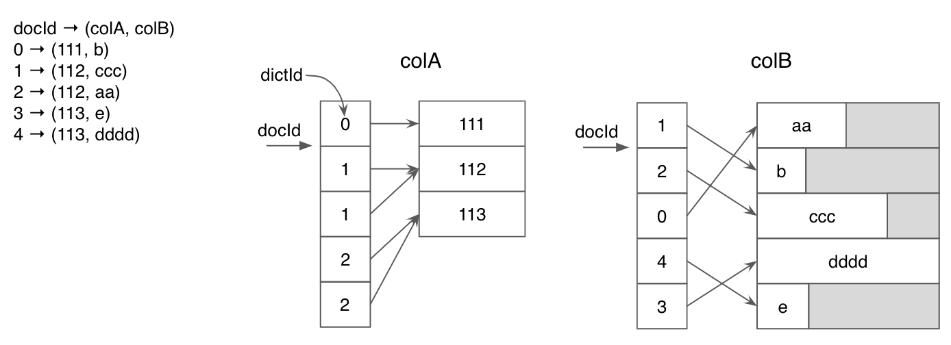
The below diagram shows the dictionary encoding for two columns with integer and string types. ForcolA, dictionary encoding saved a significant amount of space for duplicated values.
The diagram below illustrates dictionary encoding for two columns with different data types (integer and string). For colA, dictionary encoding leads to significant space savings due to duplicated values. However, for colB, which contains mostly unique values, the compression effect is limited, and padding overhead may be high.
When using the dictionary-encoded forward index for multi-value column, to further compress the forward index for repeated multi-value entires, enable the MV_ENTRY_DICT compression type which adds another level of dictionary encoding on the multi-value entries. This may be useful, for example, in cases where you pre-join a fact table with dimension table, where the multi-value entries in the dimension table are repeated after joining with the fact table.
It can be enabled with parameter:
Parameter
Default
Description
dictIdCompressionType
null
The compression that will be used for dictionary-encoded forward index
Sorted forward index with run-length encoding
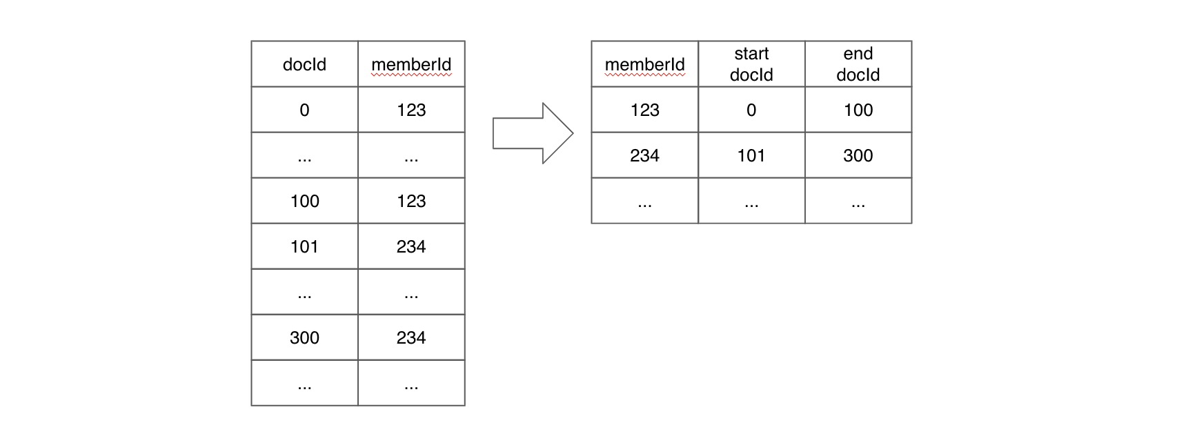
When a column is physically sorted, Pinot employs a sorted forward index with run-length encoding, which builds upon dictionary encoding. Instead of storing dictionary IDs for each document ID, this approach stores pairs of start and end document IDs for each unique value.
Sorted forward index
(For simplicity, this diagram does not include the dictionary encoding layer.)
Sorted forward indexes offer the benefits of efficient compression and data locality and can also serve as an inverted index. They are active when two conditions are met: the segment is sorted by the column, and the dictionary is enabled for that column. Refer to the dictionary documentation for details on enabling the dictionary.
When dealing with multiple segments, it's crucial to ensure that data is sorted within each segment. Sorting across segments is not necessary.
To guarantee that a segment is sorted by a particular column, follow these steps:
For real-time tables, use the tableIndexConfig.sortedColumn property. If there is exactly one column specified in that array, Pinot will sort the segment by that column upon committing.
For offline tables, you must pre-sort the data by the specified column before ingesting it into Pinot.
It's crucial to note that for offline tables, the tableIndexConfig.sortedColumn property is indeed ignored.
Additionally, for online tables, even though this property is specified as a JSON array, at most one column should be included. Using an array with more than one column is incorrect and will not result in segments being sorted by all the columns listed in the array.
When a real-time segment is committed, rows will be sorted by the sorting column and it will be transformed into an offline segment.
During the creation of an offline segment, which also applies when a real-time segment is committed, Pinot scans the data in each column. If it detects that all values within a column are sorted in ascending order, Pinot concludes that the segment is sorted based on that particular column. In case this happens on more than one column, all of them are considered as sorting columns. Consequently, whether a segment is sorted by a column or not solely depends on the actual data distribution within the segment and entirely disregards the value of the sortedColumn property. This approach also implies that two segments belonging to the same table may have a different number of sorting columns. In the extreme scenario where a segment contains only one row, Pinot will consider all columns within that segment as sorting columns.
Here is an example of a table configuration that illustrates these concepts:
Checking sort status
You can check the sorted status of a column in a segment by running the following:
Alternatively, for offline tables and for committed segments in real-time tables, you can retrieve the sorted status from the getServerMetadata endpoint. The following example is based on the Batch Quick Start:
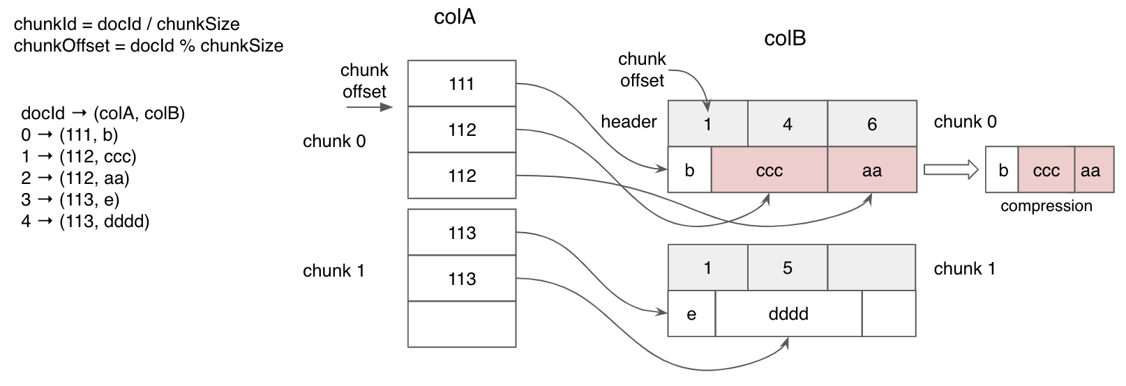
Raw value forward index
The raw value forward index stores actual values instead of IDs. This means that it eliminates the need for dictionary lookups when fetching values, which can result in improved query performance. Raw forward index is particularly effective for columns with a large number of unique values, where dictionary encoding doesn't provide significant compression benefits.
As shown in the diagram below, dictionary encoding can lead to numerous random memory accesses for dictionary lookups. In contrast, the raw value forward index allows for sequential value scanning, which can enhance query performance when applied appropriately.
When using the raw format, you can configure the following parameters:
Parameter
Default
Description
chunkCompressionType
null
The compression that will be used.
deriveNumDocsPerChunk
false
Modifies the behavior when storing variable length values (like string or bytes)
rawIndexWriterVersion
2
The version initially used
The chunkCompressionType parameter has the following valid values:
PASS_THROUGH
SNAPPY
ZSTANDARD
LZ4
LZ4_LENGTH_PREFIXED
null (the JSON null value, not "null"), which is the default. In this case, PASS_THROUGH will be used for metrics and LZ4 for other columns.
deriveNumDocsPerChunk is only used when the datatype may have a variable length, such as with string, big decimal, bytes, etc. By default, Pinot uses a fixed number of elements that was chosen empirically. If changed to true, Pinot will use a heuristic value that depends on the column data.
rawIndexWriterVersion changes the algorithm used to create the index. This changes the actual data layout, but modern versions of Pinot can read indexes written in older versions. The latest version right now is 4.
Raw forward index configuration
The recommended way to configure the forward index using raw format is by including the parameters explained above in the indexes.forward object. For example:
Deprecated
An alternative method to configure the raw format parameters is available. This older approach can still be used, although it is not recommended. Here are the details of this older method:
chunkCompressionType: This parameter can be defined as a sibling of name and encodingType in the fieldConfigList section.
deriveNumDocsPerChunk: You can configure this parameter with the property deriveNumDocsPerChunkForRawIndex. Note that in properties, all values must be strings, so valid values for this property are "true" and "false".
rawIndexWriterVersion: This parameter can be configured using the property rawIndexWriterVersion. Again, in properties, all values must be strings, so valid values for this property are "2", "3", and so on.
For example:
While this older method is still supported, it is not the recommended way to configure these parameters. There are no plans to remove support for this older method, but keep in mind that any new parameters added in the future may only be configurable in the forward JSON object.
Disabling the forward index
Traditionally the forward index has been a mandatory index for all columns in the on-disk segment file format.
However, certain columns may only be used as a filter in the WHERE clause for all queries. In such scenarios the forward index is not necessary as essentially other indexes and structures in the segments can provide the required SQL query functionality. Forward index just takes up extra storage space for such scenarios and can ideally be freed up.
Thus, to provide users an option to save storage space, a knob to disable the forward index is now available.
Forward index on one or more columns(s) in your Pinot table can be disabled with the following limitations:
Only supported for immutable (offline) segments.
If the column has a range index then the column must be of single-value type and use range index version 2.
MV columns with duplicates within a row will lose the duplicated entries on forward index regeneration. The ordering of data with an MV row may also change on regeneration. A backfill is required in such scenarios (to preserve duplicates or ordering).
If forward index regeneration support on reload (i.e. re-enabling the forward index for a forward index disabled column) is required then the dictionary and inverted index must be enabled on that particular column.
Sorted columns will allow the forward index to be disabled, but this operation will be treated as a no-op and the index (which acts as both a forward index and inverted index) will be created.
To disable the forward index, in table config under fieldConfigList, set the disabled property to true as shown below:
The older way to do so is still supported, but not recommended.
A table reload operation must be performed for the above config to take effect. Enabling / disabling other indexes on the column can be done via the usual table config options.
The forward index can also be regenerated for a column where it is disabled by enabling the index and reloading the segment. The forward index can only be regenerated if the dictionary and inverted index have been enabled for the column. If either have been disabled then the only way to get the forward index back is to regenerate the segments via the offline jobs and re-push / refresh the data.
Warning:
For multi-value (MV) columns the following invariants cannot be maintained after regenerating the forward index for a forward index disabled column:
Ordering guarantees of the MV values within a row
If entries within an MV row are duplicated, the duplicates will be lost. Regenerate the segments via your offline jobs and re-push / refresh the data to get back the original MV data with duplicates.
We will work on removing the second invariant in the future.
Examples of queries which will fail after disabling the forward index for an example column, columnA, can be found below:
Select
Forward index disabled columns cannot be present in the SELECT clause even if filters are added on it.
Group By Order By
Forward index disabled columns cannot be present in the GROUP BY and ORDER BY clauses. They also cannot be part of the HAVING clause.
Aggregation Queries
A subset of the aggregation functions do work when the forward index is disabled such as MIN, MAX, DISTINCTCOUNT, DISTINCTCOUNTHLL and more. Some of the other aggregation functions will not work such as the below:
Distinct
Forward index disabled columns cannot be present in the SELECT DISTINCT clause.
Range Queries
To run queries on single-value columns where the filter clause contains operators such as >, <, >=, <= a version 2 range index must be present. Without the range index such queries will fail as shown below:
{
  "tableName": "somePinotTable",
  "fieldConfigList": [
    {
      "name": "playerID",
      "encodingType": "RAW",
      "chunkCompressionType": "PASS_THROUGH", // it can also be defined here
      "properties": {
        "deriveNumDocsPerChunkForRawIndex": "false", // here the string value has to be used
        "rawIndexWriterVersion": "2" // here the string value has to be used
      }
    },
    ...
  ],
...
}
Geospatial data types, such as point, line and polygon;
Geospatial functions, for querying of spatial properties and relationships.
Geospatial indexing, used for efficient processing of spatial operations
Geospatial data types
Geospatial data types abstract and encapsulate spatial structures such as boundary and dimension. In many respects, spatial data types can be understood simply as shapes. Pinot supports the Well-Known Text (WKT) and Well-Known Binary (WKB) forms of geospatial objects, for example:
It is common to have data in which the coordinates are geographics or latitude/longitude. Unlike coordinates in Mercator or UTM, geographic coordinates are not Cartesian coordinates.
Geographic coordinates do not represent a linear distance from an origin as plotted on a plane. Rather, these spherical coordinates describe angular coordinates on a globe.
Spherical coordinates specify a point by the angle of rotation from a reference meridian (longitude), and the angle from the equator (latitude).
You can treat geographic coordinates as approximate Cartesian coordinates and continue to do spatial calculations. However, measurements of distance, length and area will be nonsensical. Since spherical coordinates measure angular distance, the units are in degrees.
Pinot supports both geometry and geography types, which can be constructed by the corresponding functions as shown in . And for the geography types, the measurement functions such as ST_Distance and ST_Area calculate the spherical distance and area on earth respectively.
Geospatial functions
For manipulating geospatial data, Pinot provides a set of functions for analyzing geometric components, determining spatial relationships, and manipulating geometries. In particular, geospatial functions that begin with the ST_ prefix support the SQL/MM specification.
Following geospatial functions are available out of the box in Pinot:
Aggregations
This aggregate function returns a MULTI geometry or NON-MULTI geometry from a set of geometries. it ignores NULL geometries.
Constructors
Returns a geometry type object from WKT representation, with the optional spatial system reference.
Returns a geometry type object from WKB representation.
Returns a geometry type point object with the given coordinate values.
Measurements
ST_Area(Geometry/Geography g) → double For geometry type, it returns the 2D Euclidean area of a geometry. For geography, returns the area of a polygon or multi-polygon in square meters using a spherical model for Earth.
For geometry type, returns the 2-dimensional cartesian minimum distance (based on spatial ref) between two geometries in projected units. For geography, returns the great-circle distance in meters between two SphericalGeography points. Note that g1, g2 shall have the same type.
Outputs
Returns the WKB representation of the geometry.
Returns the WKT representation of the geometry/geography.
Conversion
Converts a Geometry object to a spherical geography object.
Converts a spherical geographical object to a Geometry object.
Relationship
Returns true if and only if no points of the second geometry/geography lie in the exterior of the first geometry/geography, and at least one point of the interior of the first geometry lies in the interior of the second geometry. Warning: ST_Contains on Geography only give close approximation
ST_Equals(Geometry, Geometry) → boolean Returns true if the given geometries represent the same geometry/geography.
ST_Within(Geometry, Geometry) → boolean
Geospatial index
Geospatial functions are typically expensive to evaluate, and using geoindex can greatly accelerate the query evaluation. Geoindexing in Pinot is based on Uber’s , a hexagon-based hierarchical gridding.
A given geospatial location (longitude, latitude) can map to one hexagon (represented as H3Index). And its neighbors in H3 can be approximated by a ring of hexagons. To quickly identify the distance between any given two geospatial locations, we can convert the two locations in the H3Index, and then check the H3 distance between them. H3 distance is measured as the number of hexagons.
For example, in the diagram below, the red hexagons are within the 1 distance of the central hexagon. The size of the hexagon is determined by the resolution of the indexing. Check this table for the level of and the corresponding precision (measured in km).
How to use geoindex
To use the geoindex, first declare the geolocation field as bytes in the schema, as in the example of the .
Note the use of transformFunction that converts the created point into SphericalGeography format, which is needed by the ST_Distance function.
Next, declare the geospatial index in the you need to
Verify the dictionary is disabled (see how to ).
Enable the H3 index.
It is recommended to do the latter by using the indexes section:
Alternative the older way to configure H3 indexes is still supported:
The query below will use the geoindex to filter the Starbucks stores within 5km of the given point in the bay area.
How geoindex works
The Pinot geoindex accelerates query evaluation while maintaining accuracy. Currently, geoindex supports the ST_Distance function in the WHERE clause.
At the high level, geoindex is used for retrieving the records within the nearby hexagons of the given location, and then use ST_Distance to accurately filter the matched results.
As in the example diagram above, if we want to find all relevant points within a given distance around San Francisco (area within the red circle), then the algorithm with geoindex will:
First find the H3 distance x that contains the range (for example, within a red circle).
Then, for the points within the H3 distance (those covered by the hexagons completely within ), directly accept those points without filtering.
Finally, for the points contained in the hexagons of kRing(x)
Native text index
This page talks about native text indices and corresponding search functionality in Apache Pinot.
Native text index
Pinot supports text indexing and search by building Lucene indices as sidecars to the main Pinot segments. While this is a great technique, it essentially limits the avenues of optimizations that can be done for Pinot specific use cases of text search.
How is Pinot different?
Pinot, like any other database/OLAP engine, does not need to conform to the entire full text search domain-specific language (DSL) that is traditionally used by full-text search (FTS) engines like ElasticSearch and Solr. In traditional SQL text search use cases, the majority of text searches belong to one of three patterns: prefix wildcard queries (like pino*), postfix or suffix wildcard queries (like *inot), and term queries (like pinot).
Native text indices in Pinot
In Pinot, native text indices are built from the ground up. They use a custom text-indexing engine, coupled with Pinot's powerful inverted indices, to provide a fast text search experience.
The benefits are that native text indices are 80-120% faster than Lucene-based indices for the text search use cases mentioned above. They are also 40% smaller on disk.
Native text indices support real-time text search. For REALTIME tables, native text indices allow data to be indexed in memory in the text index, while concurrently supporting text searches on the same index.
Historically, most text indices depend on the in-memory text index being written to first and then sealed, before searches are possible. This limits the freshness of the search, being near-real-time at best.
Native text indices come with a custom in-memory text index, which allows for real-time indexing and search.
Searching Native Text Indices
The function, TEXT\_CONTAINS, supports text search on native text indices.
Examples:
TEXT\_CONTAINS can be combined using standard boolean operators
Note:TEXT\_CONTAINS supports regex and term queries and will work only on native indices. TEXT\_CONTAINS supports standard regex patterns (as used by LIKE in SQL Standard), so there might be some syntatical differences from Lucene queries.
Creating Native Text Indices
Native text indices are created using field configurations. To indicate that an index type is native, specify it using properties in the field configuration:
Indexing
This page describes the indexing techniques available in Apache Pinot
Apache Pinot supports the following indexing techniques:
Dictionary-encoded forward index with bit compression
Raw value forward index
Sorted forward index with run-length encoding
Bitmap inverted index
Sorted inverted index
Text Index
By default, Pinot creates a dictionary-encoded forward index for each column.
Enabling indexes
There are two ways to enable indexes for a Pinot table.
As part of ingestion, during Pinot segment generation
Indexing is enabled by specifying the column names in the table configuration. More details about how to configure each type of index can be found in the respective index's section linked above or in the .
Dynamically added or removed
Indexes can also be dynamically added to or removed from segments at any point. Update your table configuration with the latest set of indexes you want to have.
For example, if you have an inverted index on the foo field and now want to also include the bar field, you would update your table configuration from this:
To this:
The updated index configuration won't be picked up unless you invoke the reload API. This API sends reload messages via Helix to all servers, as part of which indexes are added or removed from the local segments. This happens without any downtime and is completely transparent to the queries.
When adding an index, only the new index is created and appended to the existing segment. When removing an index, its related states are cleaned up from Pinot servers. You can find this API under the Segments tab on Swagger:
You can also find this action on the , on the specific table's page.
Not all indexes can be retrospectively applied to existing segments. For more detailed documentation on applying indexes, see the .
Tuning Index
The inverted index provides good performance for most use cases, especially if your use case doesn't have a strict low latency requirement.
You should start by using this, and if your queries aren't fast enough, switch to advanced indices like the sorted or star-tree index.
This page describes configuring the range index for Apache Pinot
Range indexing allows you to get better performance for queries that involve filtering over a range.
It would be useful for a query like the following:
SELECT COUNT(*)
FROM baseballStats
WHERE hits > 11
A range index is a variant of an inverted index, where instead of creating a mapping from values to columns, we create mapping of a range of values to columns. You can use the range index by setting the following config in the table configuration.
Range index is supported for both dictionary and raw-encoded columns.
A good thumb rule is to use a range index when you want to apply range predicates on metric columns that have a very large number of unique values. This is because using an inverted index for such columns will create a very large index that is inefficient in terms of storage and performance.
SELECT COUNT(*) FROM Foo WHERE TEXT_CONTAINS (<column_name>, <search_expression>)
SELECT COUNT(*) FROM Foo WHERE TEXT_CONTAINS (<column_name>, "foo.*")
SELECT COUNT(*) FROM Foo WHERE TEXT_CONTAINS (<column_name>, ".*bar")
SELECT COUNT(*) FROM Foo WHERE TEXT_CONTAINS (<column_name>, "foo")
SELECT COUNT(*) FROM Foo WHERE TEXT_CONTAINS ("col1", "foo") AND TEXT_CONTAINS ("col2", "bar")
Use a timestamp index to speed up your time query with different granularities
This feature is supported from Pinot 0.11+.
Background
The TIMESTAMP data type introduced in the stores value as millisecond epoch long value.
Typically, users won't need this low level granularity for analytics queries. Scanning the data and time value conversion can be costly for big data.
A common query pattern for timestamp columns is filtering on a time range and then grouping by using different time granularities(days/month/etc).
Typically, this requires the query executor to extract values, apply the transform functions then do filter/groupBy, with no leverage on the dictionary or index.
This was the inspiration for the Pinot timestamp index, which is used to improve the query performance for range query and group by queries on TIMESTAMP columns.
Supported data type
A TIMESTAMP index can only be created on the TIMESTAMP data type.
Timestamp Index
You can configure the granularity for a Timestamp data type column. Then:
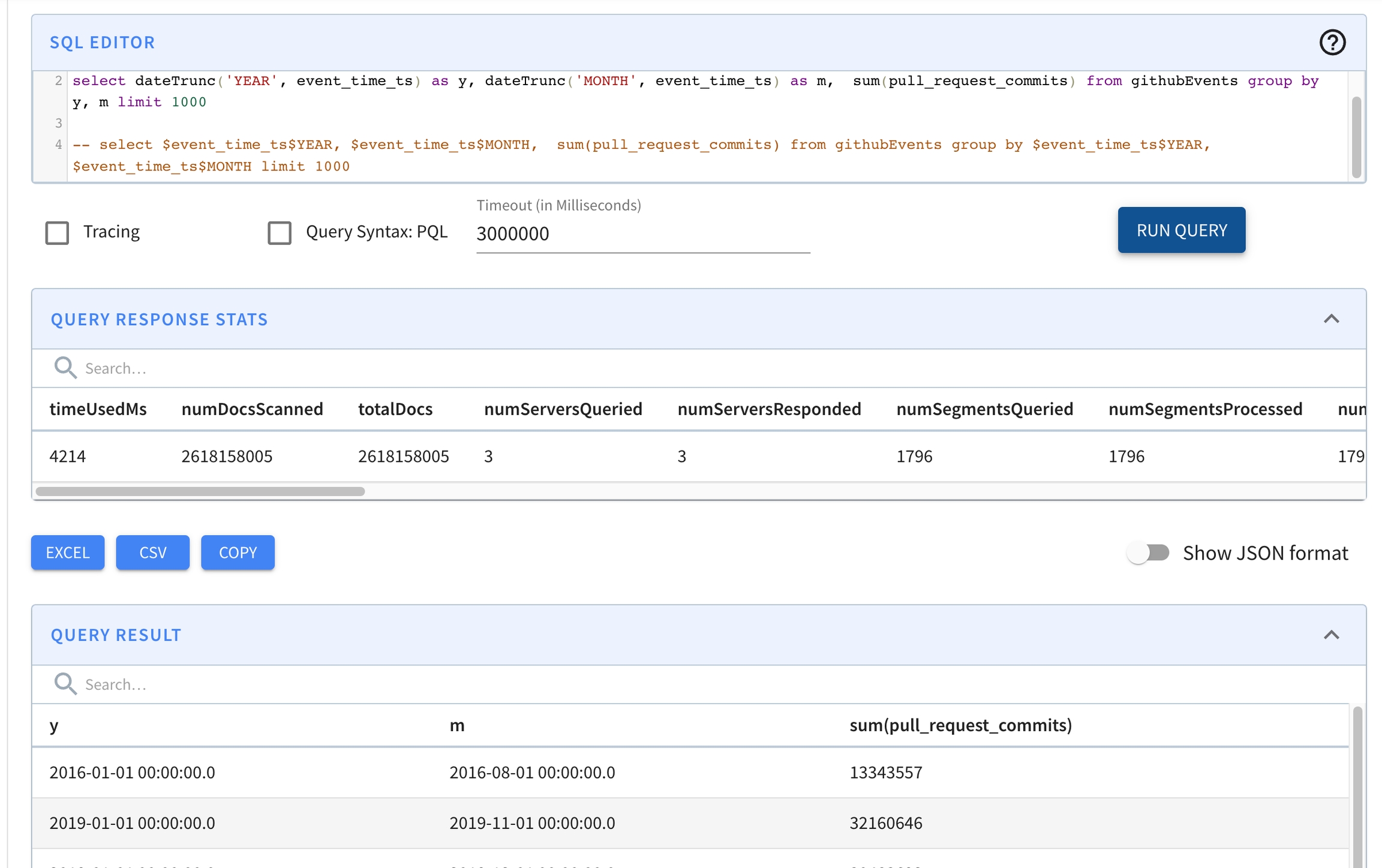
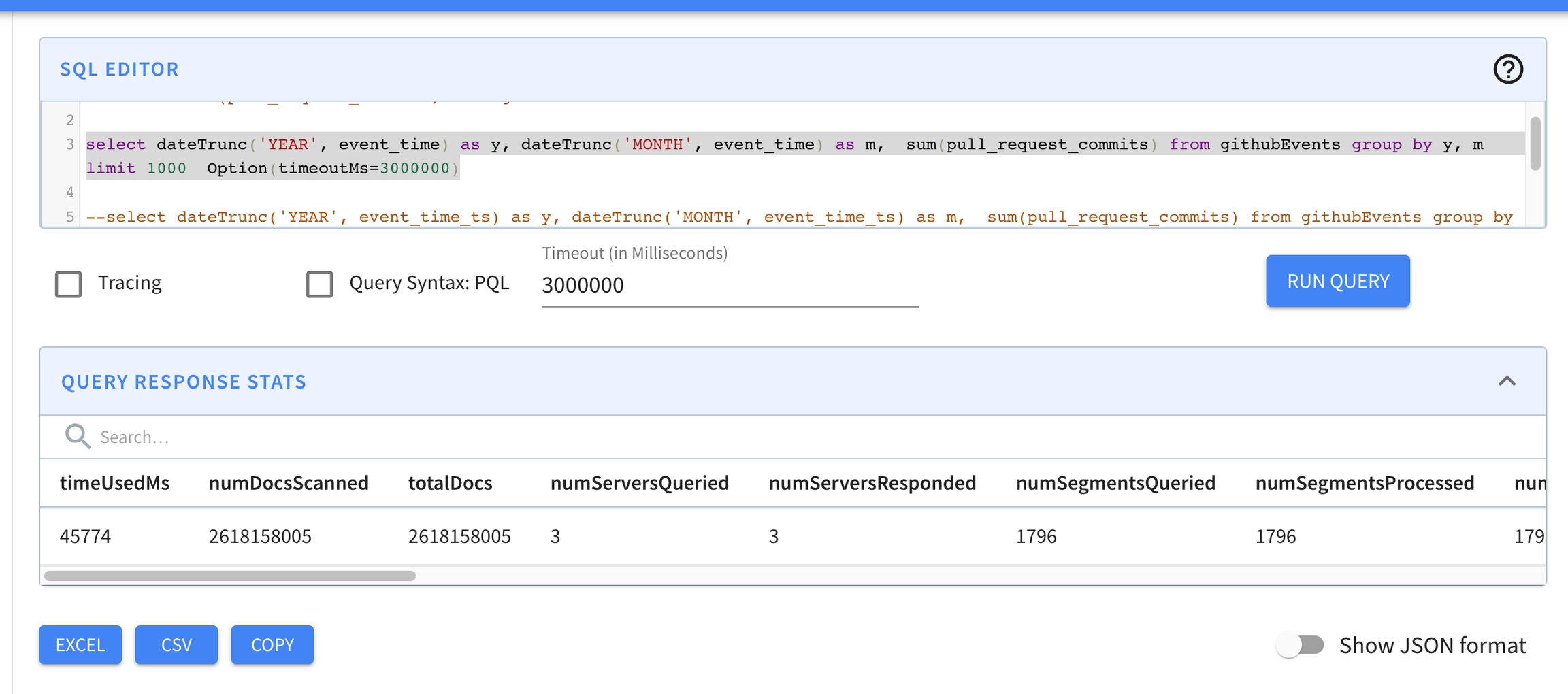
Pinot will pre-generate one column per time granularity using a forward index and range index. The naming convention is $${ts_column_name}$${ts_granularity}, where the timestamp column ts with granularities DAY, MONTH will have two extra columns generated: $ts$DAY and $ts$MONTH.
Example query usage:
Some preliminary benchmarking shows the query performance across 2.7 billion records improved from 45 secs to 4.2 secs using a timestamp index and a query like this:
vs.
Usage
The timestamp index is configured on a per column basis inside the fieldConfigList section in the table configuration.
Specify the timestampConfig field. This object must contain a field called granularities, which is an array with at least one of the following values:
MILLISECOND
SECOND
MINUTE
Sample config:
Inverted index
This page describes configuring the inverted index for Apache Pinot
We can define the forward index as a mapping from document IDs (also known as rows) to values. Similarly, an inverted index establishes a mapping from values to a set of document IDs, making it the "inverted" version of the forward index. When you frequently use a column for filtering operations like EQ (equal), IN (membership check), GT (greater than), etc., incorporating an inverted index can significantly enhance query performance.
Pinot supports two distinct types of inverted indexes: bitmap inverted indexes and sorted inverted indexes. Bitmap inverted indexes represent the actual inverted index type, whereas the sorted type is automatically available when the column is sorted. Both types of indexes necessitate the enabling of a dictionary for the respective column.
Bitmap inverted index
When a column is not sorted, and an inverted index is enabled for that column, Pinot maintains a mapping from each value to a bitmap of rows. This design ensures that value lookup operations take constant time, providing efficient querying capabilities.
When an inverted index is enabled for a column, Pinot maintains a map from each value to a bitmap of rows, which makes value lookup take constant time. If you have a column that is frequently used for filtering, adding an inverted index will improve performance greatly. You can create an inverted index on a multi-value column.
Inverted indexes are disabled by default and can be enabled for a column by specifying the configuration within the :
The older way to configure inverted indexes can also be used, although it is not actually recommended:
When the index is created
By default, bitmap inverted indexes are not generated when the segment is initially created; instead, they are created when the segment is loaded by Pinot. This behavior is governed by the table configuration option indexingConfig.createInvertedIndexDuringSegmentGeneration, which is set to false by default.
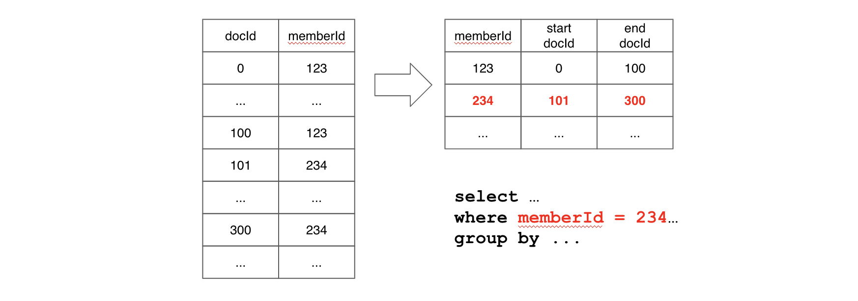
Sorted inverted index
As explained in the section, a column that is both sorted and equipped with a dictionary is encoded in a specialized manner that serves the purpose of implementing both forward and inverted indexes. Consequently, when these conditions are met, an inverted index is effectively created without additional configuration, even if the configuration suggests otherwise. This sorted version of the forward index offers a lookup time complexity of log(n) and leverages data locality.
For instance, consider the following example: if a query includes a filter on the memberId column, Pinot will perform a binary search on memberId values to find the range pair of docIds for corresponding filtering value. If the query needs to scan values for other columns after filtering, values within the range docId pair will be located together, which means we can benefit from data locality.
A sorted inverted index indeed offers superior performance compared to a bitmap inverted index, but it's important to note that it can only be applied to sorted columns. In cases where query performance with a regular inverted index is unsatisfactory, especially when a large portion of queries involve filtering on the same column (e.g., _memberId_), using a sorted index can substantially enhance query performance.
{
  "fieldConfigList": [{
    "name": "location_st_point",
    "encodingType":"RAW", // this actually disables the dictionary
    "indexTypes":["H3"],
    "properties": {
      "resolutions": "13, 5, 6" // Here resolutions must be a string with ints separated by commas
    }
  }],
  ...
}
SELECT address, ST_DISTANCE(location_st_point, ST_Point(-122, 37, 1))
FROM starbucksStores
WHERE ST_DISTANCE(location_st_point, ST_Point(-122, 37, 1)) < 5000
limit 1000
Query overwrite for predicate and selection/group by: 2.1
GROUP BY
: Functions like
dateTrunc('DAY', ts)
will be translated to use the underly column
$ts$DAY
to fetch data. 2.2
PREDICATE
: range index is auto-built for all granularity columns.
select count(*),
       datetrunc('WEEK', ts) as tsWeek
from airlineStats
WHERE tsWeek > fromDateTime('2014-01-16', 'yyyy-MM-dd')
group by tsWeek
limit 10
select dateTrunc('YEAR', event_time) as y,
       dateTrunc('MONTH', event_time) as m,
       sum(pull_request_commits)
from githubEvents
group by y, m
limit 1000
Option(timeoutMs=3000000)
This page describes configuring the JSON index for Apache Pinot.
The JSON index can be applied to JSON string columns to accelerate value lookups and filtering for the column.
When to use JSON index
Use the JSON string can be used to represent array, map, and nested fields without forcing a fixed schema. While JSON strings are flexible, filtering on JSON string columns is expensive, so consider the use case.
Suppose we have some JSON records similar to the following sample record stored in the person column:
Without an index, to look up the key and filter records based on the value, Pinot must scan and reconstruct the JSON object from the JSON string for every record, look up the key and then compare the value.
For example, in order to find all persons whose name is "adam", the query will look like:
The JSON index is designed to accelerate the filtering on JSON string columns without scanning and reconstructing all the JSON objects.
Enable and configure a JSON index
To enable the JSON index, you can configure the following options in the table configuration:
Config Key
Description
Type
Default
Recommended way to configure
The recommended way to configure a JSON index is in the fieldConfigList.indexes object, within the json key.
All options are optional, so the following is a valid configuration that use the default parameter values:
Deprecated ways to configure JSON indexes
There are two older ways to configure the indexes that can be configured in the tableIndexConfig section inside table config.
The first one uses the same JSON explained above, but it is defined inside tableIndexConfig.jsonIndexConfigs.<column name>:
Like in the previous case, all parameters are optional, so the following is also valid:
The last option does not support to configure any parameter. In order to use this option, add the name of the column in tableIndexConfig.jsonIndexColumns like in this example:
Example:
With the following JSON document:
Using the default setting, we will flatten the document into the following records:
With maxLevels set to 1:
With maxLevels set to 2:
With excludeArray set to true:
With disableCrossArrayUnnest set to true:
With includePaths set to ["$.name", "$.addresses[*].country"]:
With excludePaths set to ["$.age", "$.addresses[*].number"]:
With excludeFields set to ["age", "street"]:
Note that the JSON index can only be applied to STRING/JSON columns whose values are JSON strings.
To reduce unnecessary storage overhead when using a JSON index, we recommend that you add the indexed column to the noDictionaryColumns columns list.
For instructions on that configuration property, see the documentation.
How to use the JSON index
The JSON index can be used via the JSON_MATCH predicate: JSON_MATCH(<column>, '<filterExpression>'). For example, to find every entry with the name "adam":
Note that the quotes within the filter expression need to be escaped.
Supported filter expressions
Simple key lookup
Find all persons whose name is "adam":
Chained key lookup
Find all persons who have an address (one of the addresses) with number 112:
Nested filter expression
Find all persons whose name is "adam" and also have an address (one of the addresses) with number 112:
Array access
Find all persons whose first address has number 112:
Existence check
Find all persons who have a phone field within the JSON:
Find all persons whose first address does not contain floor field within the JSON:
JSON context is maintained
The JSON context is maintained for object elements within an array, meaning the filter won't cross-match different objects in the array.
To find all persons who live on "main st" in "ca":
This query won't match "adam" because none of his addresses matches both the street and the country.
If you don't want JSON context, use multiple separate JSON_MATCH predicates. For example, to find all persons who have addresses on "main st" and have addresses in "ca" (matches need not have the same address):
This query will match "adam" because one of his addresses matches the street and another one matches the country.
The array index is maintained as a separate entry within the element, so in order to query different elements within an array, multiple JSON_MATCH predicates are required. For example, to find all persons who have first address on "main st" and second address on "second st":
Supported JSON values
Object
See examples above.
Array
To find the records with array element "item1" in "arrayCol":
To find the records with second array element "item2" in "arrayCol":
Value
To find the records with value 123 in "valueCol":
Null
To find the records with null in "nullableCol":
Limitations
The key (left-hand side) of the filter expression must be the leaf level of the JSON object, for example, "$.addresses[*]"='main st' won't work.
includePaths
Only include the given paths, e.g. "$.a.b", "$.a.c[*]" (mutual exclusive with excludePaths). Paths under the included paths will be included, e.g. "$.a.b.c" will be included when "$.a.b" is configured to be included.
Set<String>
null (include all paths)
excludePaths
Exclude the given paths, e.g. "$.a.b", "$.a.c[*]" (mutual exclusive with includePaths). Paths under the excluded paths will also be excluded, e.g. "$.a.b.c" will be excluded when "$.a.b" is configured to be excluded.
Set<String>
null (include all paths)
excludeFields
Exclude the given fields, e.g. "b", "c", even if it is under the included paths.
Set<String>
null (include all fields)
maxLevels
Max levels to flatten the json object (array is also counted as one level)
int
-1 (unlimited)
excludeArray
Whether to exclude array when flattening the object
boolean
false (include array)
disableCrossArrayUnnest
Whether to not unnest multiple arrays (unique combination of all elements)
SELECT ...
FROM mytable
WHERE JSON_MATCH(person, '"$.name"=''adam''')
SELECT ...
FROM mytable
WHERE JSON_MATCH(person, '"$.name"=''adam''')
SELECT ...
FROM mytable
WHERE JSON_MATCH(person, '"$.addresses[*].number"=112')
SELECT ...
FROM mytable
WHERE JSON_MATCH(person, '"$.name"=''adam'' AND "$.addresses[*].number"=112')
SELECT ...
FROM mytable
WHERE JSON_MATCH(person, '"$.addresses[0].number"=112')
SELECT ...
FROM mytable
WHERE JSON_MATCH(person, '"$.phone" IS NOT NULL')
SELECT ...
FROM mytable
WHERE JSON_MATCH(person, '"$.addresses[0].floor" IS NULL')
SELECT ...
FROM mytable
WHERE JSON_MATCH(person, '"$.addresses[*].street"=''main st'' AND "$.addresses[*].country"=''ca''')
SELECT ...
FROM mytable
WHERE JSON_MATCH(person, '"$.addresses[*].street"=''main st''') AND JSON_MATCH(person, '"$.addresses[*].country"=''ca''')
SELECT ...
FROM mytable
WHERE JSON_MATCH(person, '"$.addresses[0].street"=''main st''') AND JSON_MATCH(person, '"$.addresses[1].street"=''second st''')
["item1", "item2", "item3"]
SELECT ...
FROM mytable
WHERE JSON_MATCH(arrayCol, '"$[*]"=''item1''')
SELECT ...
FROM mytable
WHERE JSON_MATCH(arrayCol, '"$[1]"=''item2''')
123
1.23
"Hello World"
SELECT ...
FROM mytable
WHERE JSON_MATCH(valueCol, '"$"=123')
null
SELECT ...
FROM mytable
WHERE JSON_MATCH(nullableCol, '"$" IS NULL')
Text search support
This page talks about support for text search in Pinot.
Why do we need text search?
Pinot supports super-fast query processing through its indexes on non-BLOB like columns. Queries with exact match filters are run efficiently through a combination of dictionary encoding, inverted index, and sorted index.
This is useful for a query like the following, which looks for exact matches on two columns of type STRING and INT respectively:
For arbitrary text data that falls into the BLOB/CLOB territory, we need more than exact matches. This often involves using regex, phrase, fuzzy queries on BLOB like data. Text indexes can efficiently perform arbitrary search on STRING columns where each column value is a large BLOB of text using the
TEXT_MATCH
function, like this:
where <column_name> is the column text index is created on and <search_expression> conforms to one of the following:
Pinot supports text search with the following requirements:
The column type should be STRING.
The column should be single-valued.
Using a text index in coexistence with other Pinot indexes is not supported.
Sample Datasets
Text search should ideally be used on STRING columns where doing standard filter operations (EQUALITY, RANGE, BETWEEN) doesn't fit the bill because each column value is a reasonably large blob of text.
Apache Access Log
Consider the following snippet from an Apache access log. Each line in the log consists of arbitrary data (IP addresses, URLs, timestamps, symbols etc) and represents a column value. Data like this is a good candidate for doing text search.
Let's say the following snippet of data is stored in the ACCESS\_LOG\_COL column in a Pinot table.
Here are some examples of search queries on this data:
Count the number of GET requests.
Count the number of POST requests that have administrator in the URL (administrator/index)
Count the number of POST requests that have a particular URL and handled by Firefox browser
Resume text
Let's consider another example using text from job candidate resumes. Each line in this file represents skill-data from resumes of different candidates.
This data is stored in the SKILLS\_COL column in a Pinot table. Each line in the input text represents a column value.
Here are some examples of search queries on this data:
Count the number of candidates that have "machine learning" and "gpu processing": This is a phrase search (more on this further in the document) where we are looking for exact match of phrases "machine learning" and "gpu processing", not necessarily in the same order in the original data.
Count the number of candidates that have "distributed systems" and either 'Java' or 'C++': This is a combination of searching for exact phrase "distributed systems" along with other terms.
Query Log
Next, consider a snippet from a log file containing SQL queries handled by a database. Each line (query) in the file represents a column value in the QUERY\_LOG\_COL column in a Pinot table.
Here are some examples of search queries on this data:
Count the number of queries that have GROUP BY
Count the number of queries that have the SELECT count... pattern
Count the number of queries that use BETWEEN filter on timestamp column along with GROUP BY
Read on for concrete examples on each kind of query and step-by-step guides covering how to write text search queries in Pinot.
A column in Pinot can be dictionary-encoded or stored RAW. In addition, we can create an inverted index and/or a sorted index on a dictionary-encoded column.
The text index is an addition to the type of per-column indexes users can create in Pinot. However, it only supports text index on a RAW column, not a dictionary-encoded column.
Enable a text index
Enable a text index on a column in the table configuration by adding a new section with the name "fieldConfigList".
Each column that has a text index should also be specified as noDictionaryColumns in tableIndexConfig:
You can configure text indexes in the following scenarios:
Adding a new table with text index enabled on one or more columns.
Adding a new column with text index enabled to an existing table.
Enabling a text index on an existing column.
When you're using a text index, add the indexed column to the noDictionaryColumns columns list to reduce unnecessary storage overhead.
For instructions on that configuration property, see the Raw value forward index documentation.
Text index creation
Once the text index is enabled on one or more columns through a table configuration, segment generation code will automatically create the text index (per column).
Text index is supported for both offline and real-time segments.
Text parsing and tokenization
The original text document (denoted by a value in the column that has text index enabled) is parsed, tokenized and individual "indexable" terms are extracted. These terms are inserted into the index.
Pinot's text index is built on top of Lucene. Lucene's standard english text tokenizer generally works well for most classes of text. To build a custom text parser and tokenizer to suit particular user requirements, this can be made configurable for the user to specify on a per-column text-index basis.
There is a default set of "stop words" built in Pinot's text index. This is a set of high frequency words in English that are excluded for search efficiency and index size, including:
Any occurrence of these words will be ignored by the tokenizer during index creation and search.
In some cases, users might want to customize the set. A good example would be when IT (Information Technology) appears in the text that collides with "it", or some context-specific words that are not informative in the search. To do this, one can config the words in fieldConfig to include/exclude from the default stop words:
The words should be comma separated and in lowercase. Words appearing in both lists will be excluded as expected.
Writing text search queries
The TEXT_MATCH function enables using text search in SQL/PQL.
TEXT_MATCH(text_column_name, search_expression)
text_column_name - name of the column to do text search on.
search_expression - search query
You can use TEXT_MATCH function as part of queries in the WHERE clause, like this:
You can also use the TEXT_MATCH filter clause with other filter operators. For example:
You can combine multiple TEXT_MATCH filter clauses:
TEXT_MATCH can be used in WHERE clause of all kinds of queries supported by Pinot.
Selection query which projects one or more columns
User can also include the text column name in select list
Aggregation query
Aggregation GROUP BY query
The search expression (the second argument to TEXT_MATCH function) is the query string that Pinot will use to perform text search on the column's text index.
Phrase query
This query is used to seek out an exact match of a given phrase, where terms in the user-specified phrase appear in the same order in the original text document.
The following example reuses the earlier example of resume text data containing 14 documents to walk through queries. In this sentence, "document" means the column value. The data is stored in the SKILLS\_COL column and we have created a text index on this column.
This example queries the SKILL\_COL column to look for documents where each matching document MUST contain phrase "Distributed systems":
The search expression is '\"Distributed systems\"'
The search expression is always specified within single quotes '<your expression>'
Since we are doing a phrase search, the phrase should be specified within double quotes inside the single quotes and the double quotes should be escaped
'\"<your phrase>\"'
The above query will match the following documents:
But it won't match the following document:
This is because the phrase query looks for the phrase occurring in the original document "as is". The terms as specified by the user in phrase should be in the exact same order in the original document for the document to be considered as a match.
NOTE: Matching is always done in a case-insensitive manner.
The next example queries the SKILL\_COL column to look for documents where each matching document MUST contain phrase "query processing":
The above query will match the following documents:
Term query
Term queries are used to search for individual terms.
This example will query the SKILL\_COL column to look for documents where each matching document MUST contain the term 'Java'.
As mentioned earlier, the search expression is always within single quotes. However, since this is a term query, we don't have to use double quotes within single quotes.
Composite query using Boolean operators
The Boolean operators AND and OR are supported and we can use them to build a composite query. Boolean operators can be used to combine phrase and term queries in any arbitrary manner
This example queries the SKILL\_COL column to look for documents where each matching document MUST contain the phrases "distributed systems" and "tensor flow". This combines two phrases using the AND Boolean operator.
The above query will match the following documents:
This example queries the SKILL\_COL column to look for documents where each document MUST contain the phrase "machine learning" and the terms 'gpu' and 'python'. This combines a phrase and two terms using Boolean operators.
The above query will match the following documents:
When using Boolean operators to combine term(s) and phrase(s) or both, note that:
The matching document can contain the terms and phrases in any order.
The matching document may not have the terms adjacent to each other (if this is needed, use appropriate phrase query).
Use of the OR operator is implicit. In other words, if phrase(s) and term(s) are not combined using AND operator in the search expression, the OR operator is used by default:
This example queries the SKILL\_COL column to look for documents where each document MUST contain ANY one of:
phrase "distributed systems" OR
term 'java' OR
term 'C++'.
Grouping using parentheses is supported:
This example queries the SKILL\_COL column to look for documents where each document MUST contain
phrase "distributed systems" AND
at least one of the terms Java or C++
Here the terms Java and C++ are grouped without any operator, which implies the use of OR. The root operator AND is used to combine this with phrase "distributed systems"
Prefix query
Prefix queries can be done in the context of a single term. We can't use prefix matches for phrases.
This example queries the SKILL\_COL column to look for documents where each document MUST contain text like stream, streaming, streams etc
The above query will match the following documents:
Regular Expression Query
Phrase and term queries work on the fundamental logic of looking up the terms in the text index. The original text document (a value in the column with text index enabled) is parsed, tokenized, and individual "indexable" terms are extracted. These terms are inserted into the index.
Based on the nature of the original text and how the text is segmented into tokens, it is possible that some terms don't get indexed individually. In such cases, it is better to use regular expression queries on the text index.
Consider a server log as an example where we want to look for exceptions. A regex query is suitable here as it is unlikely that 'exception' is present as an individual indexed token.
Syntax of a regex query is slightly different from queries mentioned earlier. The regular expression is written between a pair of forward slashes (/).
The above query will match any text document containing "exception".
Deciding Query Types
Combining phrase and term queries using Boolean operators and grouping lets you build a complex text search query expression.
The key thing to remember is that phrases should be used when the order of terms in the document is important and when separating the phrase into individual terms doesn't make sense from end user's perspective.
An example would be phrase "machine learning".
However, if we are searching for documents matching Java and C++ terms, using phrase query "Java C++" will actually result in in partial results (could be empty too) since now we are relying the on the user specifying these skills in the exact same order (adjacent to each other) in the resume text.
Term query using Boolean AND operator is more appropriate for such cases
Text Index Tuning
To improve Lucene index creation time, some configs have been provided. Field Config properties luceneUseCompoundFile and luceneMaxBufferSizeMB can provide faster index writing at but may increase file descriptors and/or memory pressure.
SELECT COUNT(*)
FROM Foo
WHERE STRING_COL = 'ABCDCD'
AND INT_COL > 2000
SELECT COUNT(*)
FROM Foo
WHERE TEXT_MATCH (<column_name>, '<search_expression>')
SELECT COUNT(*)
FROM MyTable
WHERE TEXT_MATCH(ACCESS_LOG_COL, 'GET')
SELECT COUNT(*)
FROM MyTable
WHERE TEXT_MATCH(ACCESS_LOG_COL, 'post AND administrator AND index')
SELECT COUNT(*)
FROM MyTable
WHERE TEXT_MATCH(ACCESS_LOG_COL, 'post AND administrator AND index AND firefox')
Distributed systems, Java, C++, Go, distributed query engines for analytics and data warehouses, Machine learning, spark, Kubernetes, transaction processing
Java, Python, C++, Machine learning, building and deploying large scale production systems, concurrency, multi-threading, CPU processing
C++, Python, Tensor flow, database kernel, storage, indexing and transaction processing, building large scale systems, Machine learning
Amazon EC2, AWS, hadoop, big data, spark, building high performance scalable systems, building and deploying large scale production systems, concurrency, multi-threading, Java, C++, CPU processing
Distributed systems, database development, columnar query engine, database kernel, storage, indexing and transaction processing, building large scale systems
Distributed systems, Java, realtime streaming systems, Machine learning, spark, Kubernetes, distributed storage, concurrency, multi-threading
CUDA, GPU, Python, Machine learning, database kernel, storage, indexing and transaction processing, building large scale systems
Distributed systems, Java, database engine, cluster management, docker image building and distribution
Kubernetes, cluster management, operating systems, concurrency, multi-threading, apache airflow, Apache Spark,
Apache spark, Java, C++, query processing, transaction processing, distributed storage, concurrency, multi-threading, apache airflow
Big data stream processing, Apache Flink, Apache Beam, database kernel, distributed query engines for analytics and data warehouses
CUDA, GPU processing, Tensor flow, Pandas, Python, Jupyter notebook, spark, Machine learning, building high performance scalable systems
Distributed systems, Apache Kafka, publish-subscribe, building and deploying large scale production systems, concurrency, multi-threading, C++, CPU processing, Java
Realtime stream processing, publish subscribe, columnar processing for data warehouses, concurrency, Java, multi-threading, C++,
SELECT SKILLS_COL
FROM MyTable
WHERE TEXT_MATCH(SKILLS_COL, '"Machine learning" AND "gpu processing"')
SELECT SKILLS_COL
FROM MyTable
WHERE TEXT_MATCH(SKILLS_COL, '"distributed systems" AND (Java C++)')
SELECT count(dimensionCol2) FROM FOO WHERE dimensionCol1 = 18616904 AND timestamp BETWEEN 1560988800000 AND 1568764800000 GROUP BY dimensionCol3 TOP 2500
SELECT count(dimensionCol2) FROM FOO WHERE dimensionCol1 = 18616904 AND timestamp BETWEEN 1560988800000 AND 1568764800000 GROUP BY dimensionCol3 TOP 2500
SELECT count(dimensionCol2) FROM FOO WHERE dimensionCol1 = 18616904 AND timestamp BETWEEN 1545436800000 AND 1553212800000 GROUP BY dimensionCol3 TOP 2500
SELECT count(dimensionCol2) FROM FOO WHERE dimensionCol1 = 18616904 AND timestamp BETWEEN 1537228800000 AND 1537660800000 GROUP BY dimensionCol3 TOP 2500
SELECT dimensionCol2, dimensionCol4, timestamp, dimensionCol5, dimensionCol6 FROM FOO WHERE dimensionCol1 = 18616904 AND timestamp BETWEEN 1561366800000 AND 1561370399999 AND dimensionCol3 = 2019062409 LIMIT 10000
SELECT dimensionCol2, dimensionCol4, timestamp, dimensionCol5, dimensionCol6 FROM FOO WHERE dimensionCol1 = 18616904 AND timestamp BETWEEN 1563807600000 AND 1563811199999 AND dimensionCol3 = 2019072215 LIMIT 10000
SELECT dimensionCol2, dimensionCol4, timestamp, dimensionCol5, dimensionCol6 FROM FOO WHERE dimensionCol1 = 18616904 AND timestamp BETWEEN 1563811200000 AND 1563814799999 AND dimensionCol3 = 2019072216 LIMIT 10000
SELECT dimensionCol2, dimensionCol4, timestamp, dimensionCol5, dimensionCol6 FROM FOO WHERE dimensionCol1 = 18616904 AND timestamp BETWEEN 1566327600000 AND 1566329400000 AND dimensionCol3 = 2019082019 LIMIT 10000
SELECT count(dimensionCol2) FROM FOO WHERE dimensionCol1 = 18616904 AND timestamp BETWEEN 1560834000000 AND 1560837599999 AND dimensionCol3 = 2019061805 LIMIT 0
SELECT count(dimensionCol2) FROM FOO WHERE dimensionCol1 = 18616904 AND timestamp BETWEEN 1560870000000 AND 1560871800000 AND dimensionCol3 = 2019061815 LIMIT 0
SELECT count(dimensionCol2) FROM FOO WHERE dimensionCol1 = 18616904 AND timestamp BETWEEN 1560871800001 AND 1560873599999 AND dimensionCol3 = 2019061815 LIMIT 0
SELECT count(dimensionCol2) FROM FOO WHERE dimensionCol1 = 18616904 AND timestamp BETWEEN 1560873600000 AND 1560877199999 AND dimensionCol3 = 2019061816 LIMIT 0
SELECT COUNT(*)
FROM MyTable
WHERE TEXT_MATCH(QUERY_LOG_COL, '"group by"')
SELECT COUNT(*)
FROM MyTable
WHERE TEXT_MATCH(QUERY_LOG_COL, '"select count"')
SELECT COUNT(*)
FROM MyTable
WHERE TEXT_MATCH(QUERY_LOG_COL, '"timestamp between" AND "group by"')
SELECT COUNT(*) FROM Foo WHERE TEXT_MATCH(...)
SELECT * FROM Foo WHERE TEXT_MATCH(...)
SELECT COUNT(*) FROM Foo WHERE TEXT_MATCH(...) AND some_other_column_1 > 20000
SELECT COUNT(*) FROM Foo WHERE TEXT_MATCH(...) AND some_other_column_1 > 20000 AND some_other_column_2 < 100000
SELECT COUNT(*) FROM Foo WHERE TEXT_MATCH(text_col_1, ....) AND TEXT_MATCH(text_col_2, ...)
Java, C++, worked on open source projects, coursera machine learning
Machine learning, Tensor flow, Java, Stanford university,
Distributed systems, Java, C++, Go, distributed query engines for analytics and data warehouses, Machine learning, spark, Kubernetes, transaction processing
Java, Python, C++, Machine learning, building and deploying large scale production systems, concurrency, multi-threading, CPU processing
C++, Python, Tensor flow, database kernel, storage, indexing and transaction processing, building large scale systems, Machine learning
Amazon EC2, AWS, hadoop, big data, spark, building high performance scalable systems, building and deploying large scale production systems, concurrency, multi-threading, Java, C++, CPU processing
Distributed systems, database development, columnar query engine, database kernel, storage, indexing and transaction processing, building large scale systems
Distributed systems, Java, realtime streaming systems, Machine learning, spark, Kubernetes, distributed storage, concurrency, multi-threading
CUDA, GPU, Python, Machine learning, database kernel, storage, indexing and transaction processing, building large scale systems
Distributed systems, Java, database engine, cluster management, docker image building and distribution
Kubernetes, cluster management, operating systems, concurrency, multi-threading, apache airflow, Apache Spark,
Apache spark, Java, C++, query processing, transaction processing, distributed storage, concurrency, multi-threading, apache airflow
Big data stream processing, Apache Flink, Apache Beam, database kernel, distributed query engines for analytics and data warehouses
CUDA, GPU processing, Tensor flow, Pandas, Python, Jupyter notebook, spark, Machine learning, building high performance scalable systems
Distributed systems, Apache Kafka, publish-subscribe, building and deploying large scale production systems, concurrency, multi-threading, C++, CPU processing, Java
Realtime stream processing, publish subscribe, columnar processing for data warehouses, concurrency, Java, multi-threading, C++,
C++, Java, Python, realtime streaming systems, Machine learning, spark, Kubernetes, transaction processing, distributed storage, concurrency, multi-threading, apache airflow
Databases, columnar query processing, Apache Arrow, distributed systems, Machine learning, cluster management, docker image building and distribution
Database engine, OLAP systems, OLTP transaction processing at large scale, concurrency, multi-threading, GO, building large scale systems
SELECT SKILLS_COL
FROM MyTable
WHERE TEXT_MATCH(SKILLS_COL, '"Distributed systems"')
Distributed systems, Java, C++, Go, distributed query engines for analytics and data warehouses, Machine learning, spark, Kubernetes, transaction processing
Distributed systems, database development, columnar query engine, database kernel, storage, indexing and transaction processing, building large scale systems
Distributed systems, Java, realtime streaming systems, Machine learning, spark, Kubernetes, distributed storage, concurrency, multi-threading
Distributed systems, Java, database engine, cluster management, docker image building and distribution
Distributed systems, Apache Kafka, publish-subscribe, building and deploying large scale production systems, concurrency, multi-threading, C++, CPU processing, Java
Databases, columnar query processing, Apache Arrow, distributed systems, Machine learning, cluster management, docker image building and distribution
Distributed data processing, systems design experience
SELECT SKILLS_COL
FROM MyTable
WHERE TEXT_MATCH(SKILLS_COL, '"query processing"')
SELECT SKILLS_COL
FROM MyTable
WHERE TEXT_MATCH(SKILLS_COL, 'Java')
SELECT SKILLS_COL
FROM MyTable
WHERE TEXT_MATCH(SKILLS_COL, '"Machine learning" AND "Tensor Flow"')
Machine learning, Tensor flow, Java, Stanford university,
C++, Python, Tensor flow, database kernel, storage, indexing and transaction processing, building large scale systems, Machine learning
CUDA, GPU processing, Tensor flow, Pandas, Python, Jupyter notebook, spark, Machine learning, building high performance scalable systems
SELECT SKILLS_COL
FROM MyTable
WHERE TEXT_MATCH(SKILLS_COL, '"Machine learning" AND gpu AND python')
CUDA, GPU, Python, Machine learning, database kernel, storage, indexing and transaction processing, building large scale systems
CUDA, GPU processing, Tensor flow, Pandas, Python, Jupyter notebook, spark, Machine learning, building high performance scalable systems
SELECT SKILLS_COL
FROM MyTable
WHERE TEXT_MATCH(SKILLS_COL, '"distributed systems" Java C++')
SELECT SKILLS_COL
FROM MyTable
WHERE TEXT_MATCH(SKILLS_COL, '"distributed systems" AND (Java C++)')
SELECT SKILLS_COL
FROM MyTable
WHERE TEXT_MATCH(SKILLS_COL, 'stream*')
Distributed systems, Java, realtime streaming systems, Machine learning, spark, Kubernetes, distributed storage, concurrency, multi-threading
Big data stream processing, Apache Flink, Apache Beam, database kernel, distributed query engines for analytics and data warehouses
Realtime stream processing, publish subscribe, columnar processing for data warehouses, concurrency, Java, multi-threading, C++,
C++, Java, Python, realtime streaming systems, Machine learning, spark, Kubernetes, transaction processing, distributed storage, concurrency, multi-threading, apache airflow
SELECT SKILLS_COL
FROM MyTable
WHERE text_match(SKILLS_COL, '/.*Exception/')
TEXT_MATCH(column, '"machine learning"')
TEXT_MATCH(column, '"Java C++"')
TEXT_MATCH(column, 'Java AND C++')
Star-tree index
This page describes the indexing techniques available in Apache Pinot.
In this page you will learn what a star-tree index is and gain a conceptual understanding of how one works.
Unlike other index techniques which work on a single column, the star-tree index is built on multiple columns and utilizes pre-aggregated results to significantly reduce the number of values to be processed, resulting in improved query performance.
One of the biggest challenges in real-time OLAP systems is achieving and maintaining tight SLAs on latency and throughput on large data sets. Existing techniques such as sorted index or inverted index help improve query latencies, but speed-ups are still limited by the number of documents that need to be processed to compute results. On the other hand, pre-aggregating the results ensures a constant upper bound on query latencies, but can lead to storage space explosion.
Use the star-tree index to utilize pre-aggregated documents to achieve both low query latencies and efficient use of storage space for aggregation and group-by queries.
Existing solutions
Consider the following data set, which is used here as an example to discuss these indexes:
Country
Browser
Locale
Impressions
Sorted index
In this approach, data is sorted on a primary key, which is likely to appear as filter in most queries in the query set.
This reduces the time to search the documents for a given primary key value from linear scan O(n) to binary search O(logn), and also keeps good locality for the documents selected.
While this is a significant improvement over linear scan, there are still a few issues with this approach:
While sorting on one column does not require additional space, sorting on additional columns requires additional storage space to re-index the records for the various sort orders.
While search time is reduced from O(n) to O(logn), overall latency is still a function of the total number of documents that need to be processed to answer a query.
Inverted index
In this approach, for each value of a given column, we maintain a list of document id’s where this value appears.
Below are the inverted indexes for columns ‘Browser’ and ‘Locale’ for our example data set:
Browser
Doc Id
Locale
Doc Id
For example, if we want to get all the documents where ‘Browser’ is ‘Firefox’, we can look up the inverted index for ‘Browser’ and identify that it appears in documents [1, 5, 6].
Using an inverted index, we can reduce the search time to constant time O(1). The query latency, however, is still a function of the selectivity of the query: it increases with the number of documents that need to be processed to answer the query.
Pre-aggregation
In this technique, we pre-compute the answer for a given query set upfront.
In the example below, we have pre-aggregated the total impressions for each country:
Country
Impressions
With this approach, answering queries about total impressions for a country is a value lookup, because we have eliminated the need to process a large number of documents. However, to be able to answer queries that have multiple predicates means we would need to pre-aggregate for various combinations of different dimensions, which leads to an exponential increase in storage space.
Star-tree solution
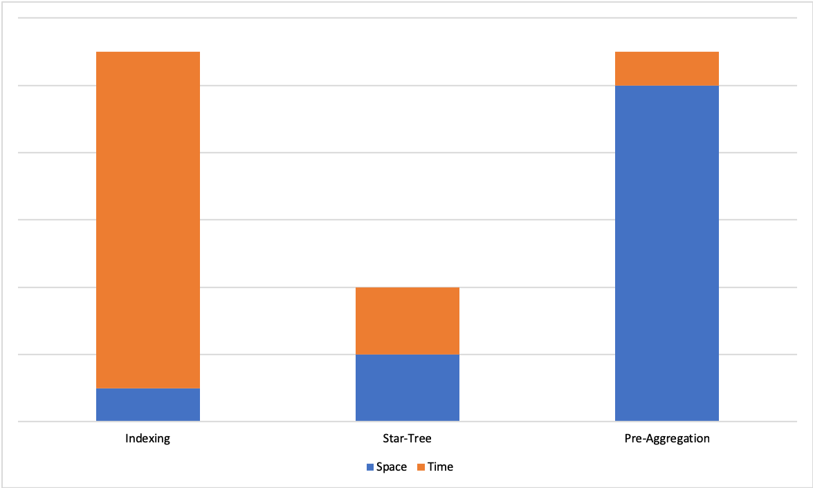
On one end of the spectrum we have indexing techniques that improve search times with a limited increase in space, but don't guarantee a hard upper bound on query latencies. On the other end of the spectrum, we have pre-aggregation techniques that offer a hard upper bound on query latencies, but suffer from exponential explosion of storage space
The star-tree data structure offers a configurable trade-off between space and time and lets us achieve a hard upper bound for query latencies for a given use case. The following sections cover the star-tree data structure, and explain how Pinot uses this structure to achieve low latencies with high throughput.
Definitions
Tree structure
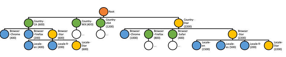
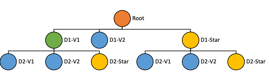
The star-tree index stores data in a structure that consists of the following properties:
Root node (Orange): Single root node, from which the rest of the tree can be traversed.
Leaf node (Blue): A leaf node can containing at most T records, where T is configurable.
Non-leaf node (Green): Nodes with more than T records are further split into children nodes.
Node properties
The properties stored in each node are as follows:
Dimension: The dimension that the node is split on
Start/End Document Id: The range of documents this node points to
Aggregated Document Id: One single document that is the aggregation result of all documents pointed by this node
Index generation
The star-tree index is generated in the following steps:
The data is first projected as per the dimensionsSplitOrder. Only the dimensions from the split order are reserved, others are dropped. For each unique combination of reserved dimensions, metrics are aggregated per configuration. The aggregated documents are written to a file and served as the initial star-tree documents (separate from the original documents).
Sort the star-tree documents based on the dimensionsSplitOrder. It is primary-sorted on the first dimension in this list, and then secondary sorted on the rest of the dimensions based on their order in the list. Each node in the tree points to a range in the sorted documents.
Aggregation
Aggregation is configured as a pair of aggregation functions and the column to apply the aggregation.
All types of aggregation function that have a bounded-sized intermediate result are supported.
Supported functions
COUNT
MIN
MAX
Unsupported functions
DISTINCT_COUNT
Intermediate result Set is unbounded.
SEGMENT_PARTITIONED_DISTINCT_COUNT:
Functions to be supported
ST_UNION
Index generation configuration
Multiple index generation configurations can be provided to generate multiple star-trees. Each configuration should contain the following properties:
Property
Description
`functionColumnPairs` and `aggregationConfigs` are interchangeable. Consider using `aggregationConfigs` since it supports additional parameters like compression.
AggregationConfigs
All aggregations of a query should be included in `aggregationConfigs` or in `functionColumnPairs` in order to use the star-tree index.
Property
Description
Default index generation configuration
A default star-tree index can be added to a segment by using the boolean config enableDefaultStarTree under the tableIndexConfig.
A default star-tree will have the following configuration:
All dictionary-encoded single-value dimensions with cardinality smaller or equal to a threshold (10000) will be included in the dimensionsSplitOrder, sorted by their cardinality in descending order.
All dictionary-encoded Time/DateTime columns will be appended to the _dimensionsSplitOrder _following the dimensions, sorted by their cardinality in descending order. Here we assume that time columns will be included in most queries as the range filter column and/or the group by column, so for better performance, we always include them as the last elements in the dimensionsSplitOrder.
Example
For our example data set, in order to solve the following query efficiently:
We may config the star-tree index as follows:
Note: In above config maxLeafRecords is set to 1 so that all of the dimension combinations are pre-aggregated for clarity in the visualization below.
Alternatively using aggregationConfigs instead of functionColumnPairs and enabling compression on the aggregation:
The star-tree and documents should be something like below:
Tree structure
The values in the parentheses are the aggregated sum of Impressions for all the documents under the node.
Star-tree documents
Country
Browser
Locale
SUM__Impressions
Query execution
For query execution, the idea is to first check metadata to determine whether the query can be solved with the star-tree documents, then traverse the Star-Tree to identify documents that satisfy all the predicates. After applying any remaining predicates that were missed while traversing the star-tree to the identified documents, apply aggregation/group-by on the qualified documents.
The algorithm to traverse the tree can be described as follows:
Start from root node.
For each level, what child node(s) to select depends on whether there are any predicates/group-by on the split dimension for the level in the query.
If there is no predicate or group-by on the split dimension, select the Star-Node if exists, or all child nodes to traverse further.
In scenarios where you have a transform on a column(s) which is in the dimension split order then Star-Tree index will still be applied. For e.g if query has round(colA,600)as roundedValue and colA is in the split order then Pinot will use the pre-aggregated records to first scan matching records and then apply transform functionround() on top to get roundedValue output.
There is a known bug which can mistakenly apply a star-tree index to queries with the OR operator on top of nested AND or NOT operators in the filter that cannot be solved with star-tree, and cause wrong results. E.g. SELECT COUNT(*) FROM myTable WHERE (A = 1 AND B = 2) OR A = 2. This bug affects release 0.9.0, 0.9.1, 0.9.2, 0.9.3, 0.10.0.
es
300
MX
Safari
en
100
USA
Chrome
en
600
USA
Firefox
es
200
USA
Firefox
en
400
Star node (Yellow): Non-leaf nodes can also have a special child node called the star node. This node contains the pre-aggregated records after removing the dimension on which the data was split for this level.
Dimensions split order ([D1, D2]): Nodes at a given level in the tree are split into children nodes on all values of a particular dimension. The dimensions split order is an ordered list of dimensions that is used to determine the dimension to split on for a given level in the tree.
The tree structure can be created recursively (starting at root node) as follows:
If a node has more than T records, it is split into multiple children nodes, one for each value of the dimension in the split order corresponding to current level in the tree.
A star node can be created (per configuration) for the current node, by dropping the dimension being split on, and aggregating the metrics for rows containing dimensions with identical values. These aggregated documents are appended to the end of the star-tree documents.
If there is only one value for the current dimension, a star node won’t be created because the documents under the star node are identical to the single node.
The above step is repeated recursively until there are no more nodes to split.
Multiple star-trees can be generated based on different configurations (dimensionsSplitOrder, aggregations, T)
SUM
AVG
MIN_MAX_RANGE
DISTINCT_COUNT_HLL
PERCENTILE_EST
PERCENTILE_TDIGEST
DISTINCT_COUNT_BITMAP
NOTE: The intermediate result RoaringBitmap is not bounded-sized, use carefully on high cardinality columns.
DISTINCT_COUNT_HLL
DISTINCT_COUNT_RAW_HLL
DISTINCT_COUNT_THETA_SKETCH
DISTINCT_COUNT_RAW_THETA_SKETCH
DISTINCT_COUNT_TUPLE_SKETCH
DISTINCT_COUNT_RAW_INTEGER_SUM_TUPLE_SKETCH
SUM_VALUES_INTEGER_SUM_TUPLE_SKETCH
AVG_VALUE_INTEGER_SUM_TUPLE_SKETCH
DISTINCT_COUNT_CPC_SKETCH
DISTINCT_COUNT_RAW_CPC_SKETCH
DISTINCT_COUNT_ULL
DISTINCT_COUNT_RAW_ULL
Intermediate result Set is unbounded.
PERCENTILE
Intermediate result List is unbounded.
Include COUNT(*) and SUM for all numeric metrics in the functionColumnPairs.
Use default maxLeafRecords (10000).
en
100
MX
Safari
es
300
USA
Chrome
en
600
USA
Firefox
en
400
USA
Firefox
es
200
CA
*
en
400
CA
*
fr
200
CA
*
*
600
MX
Safari
*
400
USA
Firefox
*
600
USA
*
en
1000
USA
*
es
200
USA
*
*
1200
*
Chrome
en
1000
*
Firefox
en
400
*
Firefox
es
200
*
Firefox
fr
200
*
Firefox
*
800
*
Safari
en
100
*
Safari
es
300
*
Safari
*
400
*
*
en
1500
*
*
es
500
*
*
fr
200
*
*
*
2200
If there are predicate(s) on the split dimension, select the child node(s) that satisfy the predicate(s).
If there is no predicate, but there is a group-by on the split dimension, select all child nodes except Star-Node.
Recursively repeat the previous step until all leaf nodes are reached, or all predicates are satisfied.
Collect all the documents pointed by the selected nodes.
If all predicates and group-by's are satisfied, pick the single aggregated document from each selected node.
Otherwise, collect all the documents in the document range from each selected node.note
CA
Chrome
en
400
CA
Firefox
fr
200
MX
Firefox
1,5,6
Chrome
0,4
Safari
2,3
en
0,3,4,6
es
2,5
fr
1
CA
600
MX
400
USA
1200
dimensionsSplitOrder
An ordered list of dimension names can be specified to configure the split order. Only the dimensions in this list are reserved in the aggregated documents. The nodes will be split based on the order of this list. For example, split at level i is performed on the values of dimension at index i in the list.
- The star-tree dimension does not have to be a dimension column in the table, it can also be time column, date-time column, or metric column if necessary.
- The star-tree dimension column should be dictionary encoded in order to generate the star-tree index.
- All columns in the filter and group-by clause of a query should be included in this list in order to use the star-tree index.
skipStarNodeCreationForDimensions
(Optional, default empty): A list of dimension names for which to not create the Star-Node.
functionColumnPairs
A list of aggregation function and column pairs (split by double underscore “__”). E.g. SUM__Impressions (SUM of column Impressions) or COUNT__*.
(Optional, default 10000): The threshold T to determine whether to further split each node.
columnName
(Required) Name of the column to aggregate. The column can be either dictionary encoded or raw.
aggregationFunction
(Required) Name of the aggregation function to use.
compressionCodec
(Optional, default PASS_THROUGH) Used to configure the compression enabled on the star-tree-index. Useful when aggregating on columns that contain big values. For example, a BYTES column containing HLL counters serialisations used to calculate DISTINCTCOUNTHLL. In this case setting "compressionCodec": "LZ4" can significantly reduce the space used by the index.
CA
Chrome
en
400
CA
Firefox
fr
200
MX
Star-tree index structure
Safari
Safari
SELECT SUM(Impressions)
FROM myTable
WHERE Country = 'USA'
AND Browser = 'Chrome'
GROUP BY Locale